Trick to enhance power of Regression model
We, as analysts, specialize in optimization of already optimized processes. As the optimization gets finer, opportunity to make the process better gets thinner. One of the predictive modeling technique used frequently use is regression (Linear or Logistic). Another equally competing technique (typically considered as a challenger) is Decision tree.
What if we could combine the benefits of both the techniques to create powerful predictive models?

The trick mentioned in this article does exactly that and can help you improve model lifts by as high as 120%.
[stextbox id=”section”]Overview of both the modeling techniques[/stextbox]
Before getting into details of this trick, let me touch up briefly on pros and cons of the two mentioned techniques. If you want to read basics of predictive modeling, click here.
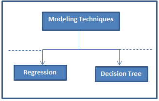
- Regression assumes continuous variable as is and generates a prediction through fitting curves for each combination input variables.
- Decision tree (CART/CHAID), on the other hand, converts these continuous variables into buckets and thereby segments the overall population.
Converting variables into buckets might make the analysis simpler, but it makes the model lose some predictive power because of its indifference for data points lying in the same bucket.
[stextbox id=”section”]A simple case study to understand pros and cons of the two techniques[/stextbox]
If decision tree losses such an important trait, how come it has a predictive power similar to that of a regression model? It is because it captures the covariance term effectively, which makes a decision tree stronger. Say, we want to find probability of a person to buy a BMW.
Decision tree:
A decision tree simply segments the population in as discrete buckets as possible. This is how a typical decision tree would look like:
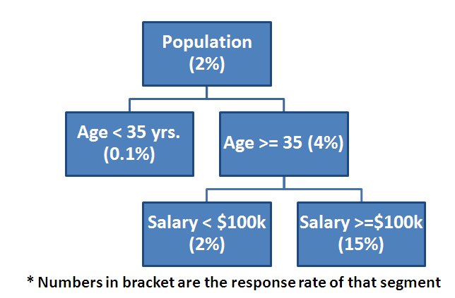
Even though the tree does not distinguish between Age 37 yrs. and 90 yrs. or salary $150k and $1M, the covariance between Age and Salary is making the decision tree’s prediction powerful.
Regression model:
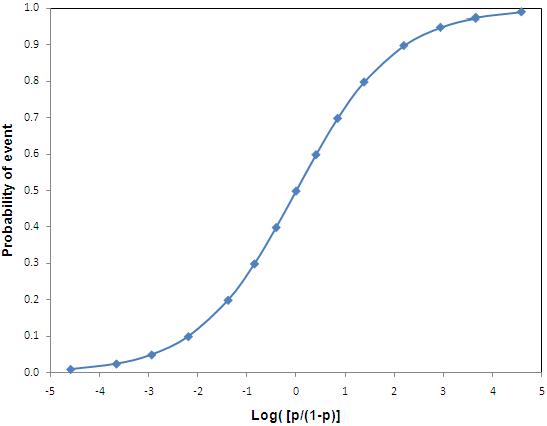
On the other hand, logistic regression makes use of Logit function (shape below) to create prediction. A typical equation would look like this:
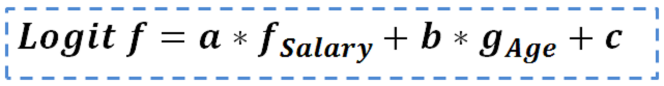
where a, b and c are constants
[stextbox id=”section”]Industry standard techniques to address shortcomings of regression modeling:[/stextbox]
There are two basic techniques to capture covariance and discontinuity of the target variable:
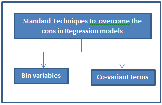
- Bin variable with discontinuous relation: This is a technique used in almost all the models. If you are not familiar with this technique, it is nothing but flagging variables in the interval where a strong input variable shows a discontinuous relationship with the output variable.For example, 10% people break at least0 one traffic signal in US everyday. Only 3% of households with salary between $70k and $100k break traffic signal. Whereas, 11% of the rest of the population break traffic signal everyday, and this is almost uniformly distributed. In this case, to predict the propensity to break the signal, a good variable can be the salary bin $70k to $100k.
- Introduce covariance variables: This is a technique used rarely. The reason being such variables are very difficult to comprehend and difficult to explain business.
Each of these techniques capture co-variance and discontinuous variable well.
However, consider the following scenario where these approach have a high propensity to fail:
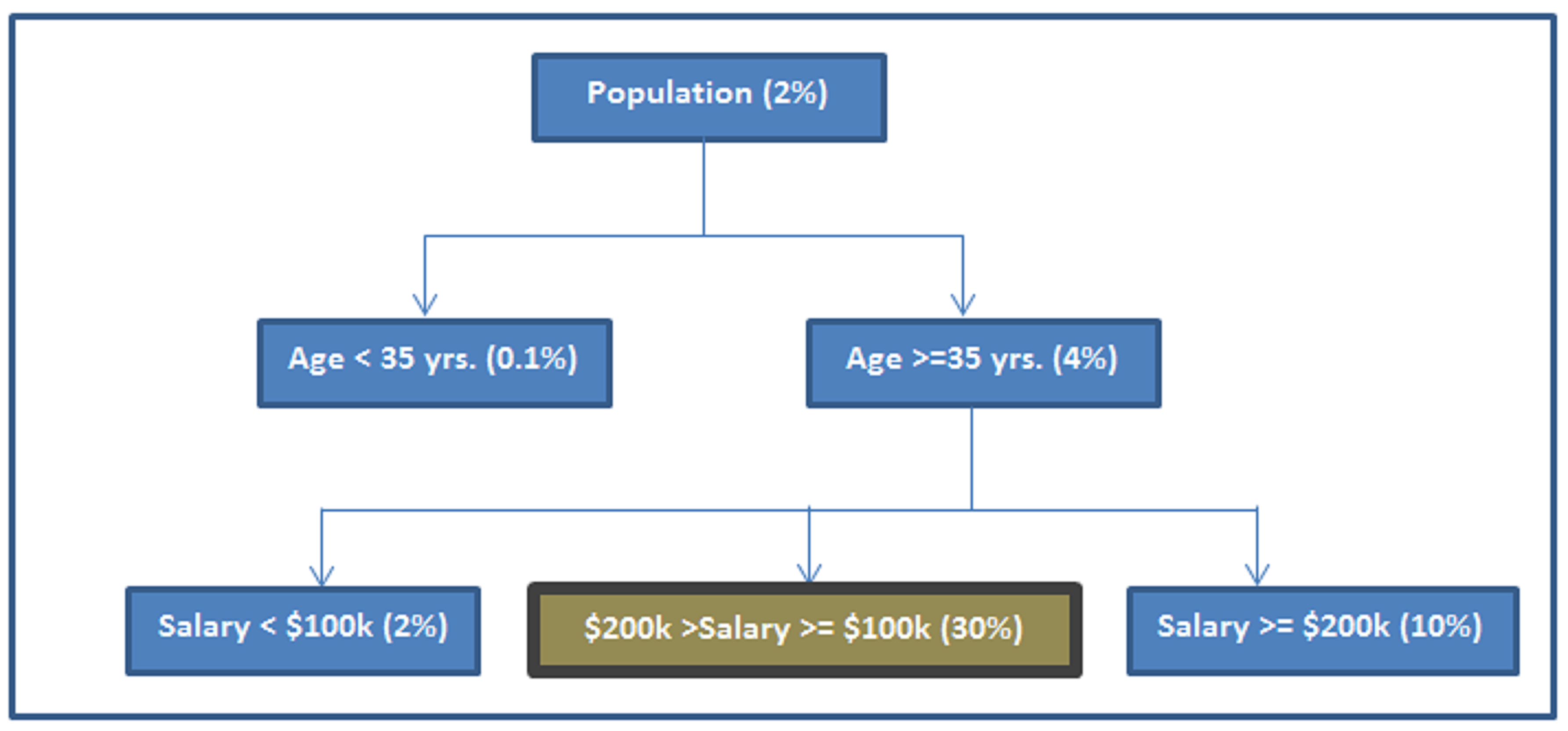
Say in the population discussed in last section, people with salary between $100 K and $200 K and age above 35 years form a segment with exceptionally high BMW take up rate (30%). If we use the two discussed techniques, will the model capture this exceptionally high take-up segment? Will regression still be a better model compared to decision tree?
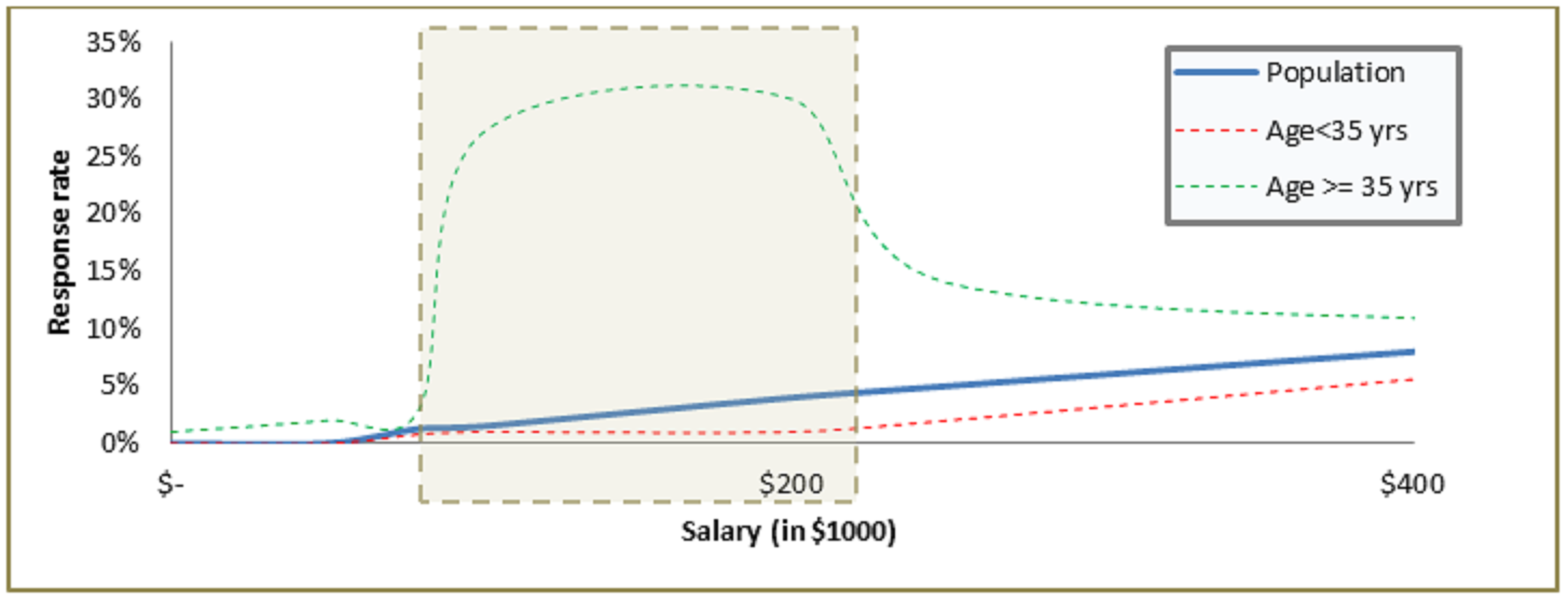
The answer is NO and NO, the regression will not be able to effectively capture this segment. Why does bin technique not capture this? The reason is that binning is done on a one-dimensional variable and in overall population salary bracket $100k to $200k might not even be different from rest. As you can see in the figure above, the response rate of the income bucket $100k to $200k is not differentiated when analyzed on overall population. But this bucket becomes very different when an initial cut of age >=35yrs is added.
Why does covariance term fail as well? The overall covariance between age and salary might not be significant for the overall population. Hence to have higher predictive power, the model needs an input that the trends of a particular segment are significantly different from rest of the population. Therefore,when the two problems i.e. discontinuity and covariance, exist simultaneously, regression model fails to capture the hidden segment. Decision tree, on the other hand works very well in these scenarios.
[stextbox id=”section”]Have you guessed the trick?[/stextbox]
Having worked on many of such problems, I find the following solution very handy. Both regression and decision tree have pros. Why not combine the pros of the two methods? I have used this technique in a number of models. And I was pleasantly surprised by the additional predictive power I got every time. There are two ways to combine the two methods:
- Introduce a new Covariant Variable: A faster and an effective way to use the tool. Simply add this as one of the input variable for the logistic model.This Covariant term (a bi-variant bin) can be defined as:
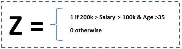
- Make two alternative models: A time taking but more effective method in case the exceptional bin has reasonable size. In this method we build two regression models separately for the identified bin (Age > 35yrs. and $200k > Salary > $100k ) and the rest of population. And add the two function by following logic.
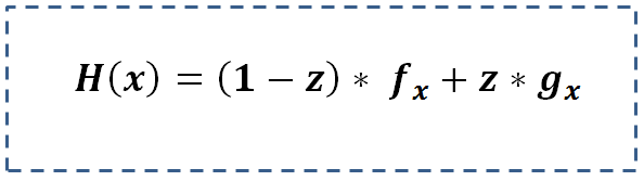
Here, g(x) is the equation for the identified bin and f(x) is the equation for rest of the population. Z is same as defined in the last block.
I am sure you are wondering “What makes the lift go even higher than the lifts you saw in the two models?” If you are not I will really like to know your opinions on the reason.
[stextbox id=”section”]How does it work? How do this trick create such impactful results?[/stextbox]
Now let’s try to think about what did we just do? Decision tree was coming out to be a better model because of a hidden pocket, which was two-dimensional bin. Even with the limitation of not using the continuous behavior of interval variable decision tree became very efficient to reduce false positive in a particular segment. By introducing the flag of this segment in logistic regression we have given the regression the additional dimension decision tree was able to capture. Hence by additionally using the continuous behavior of interval variables such as age, salary the new logistic regression becomes stronger than the decision tree.
[stextbox id=”section”]Constraints of this trick:[/stextbox]
There are two major constraints of using this technique,
- Multi-collinearity: For models, where the VIF factor becomes unacceptable, the number of variables used to create the new input function should be reduced.
- High Covariance: When overall covariance between two terms is high, this technique simply fails. This is because we will have to create too many buckets and , therefore, too many variables to be introduced in the regression model. This will introduce very high collinearity to the regression.
In general, I follow a thumb rule of not making more than 6 leaves in the parent tree. This, first of all, captures the most important co-variant buckets and does not introduce the two mentioned problems. Also, make sure the final bucket makes sense with business and is not merely a noise.
[stextbox id=”section”]Final notes:[/stextbox]
This trick helped me make my lifts rise by as high as 120% of the original lift. The best part of this trick is that it gives you a good starting point for your regression where you start with a couple of already proved significant variables.
What do think of this technique? Do you think this provides solution to any problem you face? Are there any other techniques you use to improve performance of your models (prediction or stability)? Do let us know your thoughts in comments below.
If you like what you just read & want to continue your analytics learning, subscribe to our emails or like our facebook page.
Tavish Srivastava, co-founder and Chief Strategy Officer of Analytics Vidhya, is an IIT Madras graduate and a passionate data-science professional with 8+ years of diverse experience in markets including the US, India and Singapore, domains including Digital Acquisitions, Customer Servicing and Customer Management, and industry including Retail Banking, Credit Cards and Insurance. He is fascinated by the idea of artificial intelligence inspired by human intelligence and enjoys every discussion, theory or even movie related to this idea.


Hi Kunal, If I follow the equation given in step 2 to compute H(x) then is it not the same as combining f(x) and g(x)? Because, z value for g(x) will always be 1 and same for f(x) will always be 0 meaning 1-z is again always 1. Is my understanding correct? Best Regards, Samarendra
Samarendra, Let me try and explain. When age > 35 for specific income, z = 1. In this case H(x) = g(x) When becomes 0, H(x) = f(x). Hence, H(x) ends up becoming a combination of 2 models. Hope this becomes clear. Kunal
Kunal, Thanks for clarifying. Then if my understanding is correct, it will not be a combination of both the model which is fine considering that a case will exclusively fall in any of the two group. Sounds interesting to me. I will try to implement it in some real-life data. Thanks again for sharing this. Samarendra
Tavish, you are assuming discontinuity, but in reading the article it seems to me discontinuity was artifically imposed by the analyst. CART (and its ilks) is inefficient not just because of issues you mentioned, but also because it hardly provides stable results. There's absolutely no reason to bin continuous variables which will lead to oversimplifications, besides implicitly assuming that the misclassification cost is the same. I suspect that might be one of the reasons why you are getting similar prediction errors when using logistic vs. CART. A sensible logistic model with no linearity assumptions and appropriate penalization and shrinkage will almost always produce superior results to CART and the likes.
Thomas, I completely agree that regression with non-linearity assumption will give superior result because for obvious reason, Linear regression is a subset of non-linear regression. But the motive of the article was that even non linear regression can be enhanced by introducing multi-variant bin variable. This multi-variant bin variables can be generated by plotting a simple decision tree.
I think you can achieve this in SAS EM in similar way. First you fit a decision tree and then output the leaf node number (nominal) as one input variables to the sub-sequent regression model. So you model would like Y=X*Beta + xl*Lead_number. My worry is same as yours, original X matrix is highly correlated with the xl. Multicollinearity would become a problem.
Hongbing, You are right. SAS EM does have that functionality. I use to do the same but in general it leads to multi-collinearity because the tree is too exhaustive. To combat this problem you can make an interactive tree only to 4-6 leafs and then add the regression node. Nonetheless, you are correct, the same can be achieved directly by E-Miner.
Thank you for your very cogent explanation here. Some may know this phenomenon as "testing for interaction terms", very commonly done in epidemiology and public health statistics (use your example, instead of "buying a BMW, think "having a good health outcome", based on an interaction between gender and age, or age and a chronic disease. When the interaction is significant, final models can be created within each age-sex group, or stratified outcomes can be presented to the audience to make it apparent what is going on. Interaction terms can easily be specified in any SAS model, too. I liked seeing this comparison to the differences between using regression and decision trees. Maybe this is helpful, maybe not, depending on training and subject matter.
Interesting post Tavish! But a point to note is that binning continuous variables is not the most efficient solution and I don't think it will provide superior information. From a purely statistical perspective you are coarsening the information and this invariably should not be helpful. If you suspect the behavior of the variable is kinky then using a spline regression may be a good solution. Alternatively if you suspect wider non linearity then rather than use logit you could think of alternative approaches like Generalized Additive Models (GAM's).My two cents!!
Hi - I have build a linear regression as well as a logistic regression model using the same dataset. In both cases, i have changed the definition of the target. As we are still not sure how we would be implementing the final model. Now the results from both models are very close. Is there a way wherein i can combine the 2 models in order to increase the predictive power of the resultant model? thanks in advance for the reply.
hi, do you have any experience with support vector machines (AI)?? I need some help,thanks
Great article, Tavish !! However, I have a couple of questions here. How is the income bracket ( > 200 k & <= 100 k ) deduced, considering the fact that this income bracket did not turn up while creating a decision tree. Also, how would the results be interpreted after executing logistic regression with an interaction variable ( Z, here). How do we explain output of the model in business terms with respect to a unit change in interaction variable.
The popular/important predictor variables that are discovered using the linear model and decision are quite different. Linear models allow us to eliminate the least significant variables. However the decision tree may tell us another story. The variable.importance function in rpart package returns us the most important variables. Decision trees are less sensitive to outliers and missing values compared to a linear model. In that case, we could use those variables from the decision tree in the linear model. Wouldn't this be more efficient?