About some time back, we hired a smart analyst in our team (let’s call him Sam). Sam’s role required him to create and maintain various financial & business models in Excel. He seemed to be on top of his game! Within 2 months of his joining, he had created 2 new models, both of them had very neat interfaces and seemed to work impeccably – really good achievement for a new member in the team.

Sadly, the models fell apart as soon as there were a few additions in the products. When the results looked unexpected, Sam was called upon to investigate what went wrong!

Sam (like a lot of analysts I have met in past), had created Excel charts and Pivot tables on static data source. So, every time the underlying data changed, the data source had to be corrected at multiple sources for the model to work again!

There are multiple problems associated with these fixed data source models in Excel:

1. The amount of time required to refresh the model in new scenarios ends up taking a lot more time than what it should ideally take.
2. The more the places where we need to update the data source, the higher the chances of making a manual error.

Fortunately, there are multiple simple ways to definedynamic ranges in Excel such that your Pivot tables and charts can reflect the changes in the size and shape of the data automatically. I’ll share a couple of these tricks in this post.

Dataset:

Let us take a simple data set (shown on the right) on which we want to create: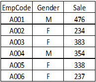

a)      A pivot table (showing gender wise Sum of Sales),

b)      A column chart (Employee code on category axis and Sales on value axis)

We want that any changes in the dataset should get reflected on charts and pivots automatically.

How to Create dynamic range in excel?

The methods to create dynamic ranges can be classified in two broad categories:

1. By use of Excel Tables
2. By defining the dynamic Range by use of Excel functions (Indirect / Offset / Index)

Method 1 – Create Dynamic range with Excel Tables

This is probably the simplest trick to achieve the desired results. Excel tables were added as a feature in Excel 2007. In excel table, we can add or remove rows or columns and it applies the formatting, formulae and filters to new rows or columns. This automatically makes our models dynamic in nature.

How to create Excel Tables?

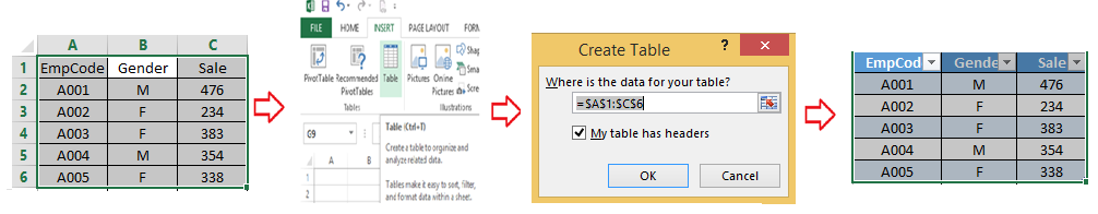
Step – 1: First select the data range that you want to convert to an excel table

Step – 2: Go to INSERT tab of the ribbon and select TABLE. Excel asks whether your table has header row or not. You should select the box, if this is the case and click OK.

Your Excel table is ready.

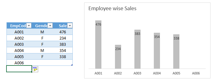
Whenever you create charts or pivot tables with excel tables, theyautomatically get updated with the addition or deletion of row/column.

In Below snapshot, you can see that as I have added a value A006 for EmpCode, it has created respective category on x-axis automatically.

Method 2 – Defining Name to dynamic Range by using Excel functions (Indirect / Offset / Index):

In the remaining article, I will explain creation of dynamic range using Index function. We will see the use of two other functions to create dynamic range in a future post.

Introduction to INDIRECT() function:

INDIRECT is used to indirectly reference a cell in a worksheet. In simple words, this function helps to put the address of one cell to another, and get data from the one cell by referencing the other.  For example, if cell B2 has the value “A1” and I have put =INDIRECT (B2) in cell C1 then this function will return the value of A1 in C1.

Syntax of INDIRECT() function:

Indirect (Ref_Text [, a1])

Ref_Text is a valid cell reference, range or defined range name like A1, A1:B3, Range1. It must be in string format.

True/False (a1) is optional parameter and default value is TRUE. It defines what style of cell reference is contained in the Ref_text argument. TRUE for A1 style (absolute referencing) and FALSE for R1C1 style (relative referencing).

Examples cases for use of INDIRECT() function:

Let’s look at the snapshot below –on the left side, we have Formula view and result view on the right.

Case 1: We have put the formula =Indirect (B2) in cell C2 and we can see that cell B2 has value A1. Now this function will retrieve the value of cell A1 in cell C2 and you can see in the result window, it is showing 1.

Case 2:Calculate the sum of A1:A5 by passing range as a string. In cell A6, We have done the sum of A1:A5 by passing it as a range where as in cell B6 we have passed the range as a string. Here indirect function has converted the range string to the table range.

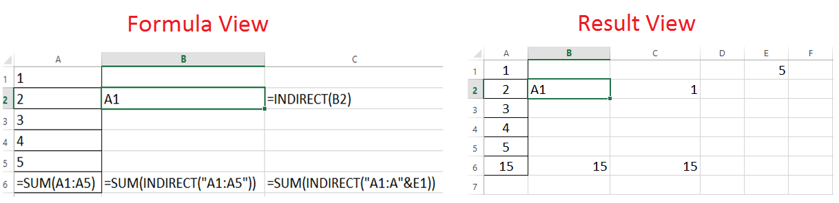
Case 3: As we know that we can pass range as a string so we can also play with column and row index by manipulating or referring to another cell value.

We have used this method to derive a formula in cell C6.You can see that the range upper row index is dependent on value of cell E1 (visible in the Result View). If Cell E1 has value 5 then the range would be A1:A5 and if it is 4 then the range would be A1:A4.

Based on this method, we can define a dynamic range, we need to find the upper limit of row and column with the help of other functions.

Define Name of Dynamic Range

Let’s say we want to define name for range A1:C6 but whenever there is addition or deletion of rows, the name range must refer the modified data range automatically.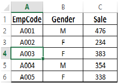

Here we will use one of the above discussed function to define named range for data available on Sheet2.

Step -1: Go to the Formula tab of ribbon and select “Define Name”.

Step -2:  Give a name to the range, here I have given “Range1” and in “refers to”box write the formula for dynamic range. Whenever we are writing formula in “refers to”, we should reference cell with sheet name like here:

=INDIRECT (“Sheet2!$A$1:$C$”&COUNTA (Sheet2!$C:$C))

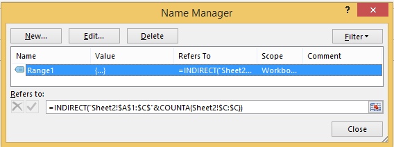
This will automatically find the reference of last row of range with the help of COUNTA and I assumed that it has information till column C only. We can also find dynamically the column index.

Create a Pivot Table with Dynamic Range Name

Step-1 First define the dynamic range name(as explained above)

Step-2 Go to insert tab and select Pivot table command. Here provide the same name of the dynamic range defined in Step 1 or press F3 key (it will show all the available range names) and select the name.

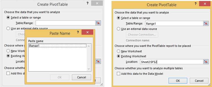
Step-3 Select the Location, where you want to place the pivot table and then click OK. Now select the dimension and values for pivot.

Here we have created a pivot table with dynamic range. Now if we add or delete rows in a given range, data range of pivot table will change automatically. We will still need to refresh the pivot tables.

Create an Excel Chart with Dynamic Range Name

Now we are going to create a column chart to look at Sales by each employee. Here EmpCode is on the category axis (X-axis) and Sales on Value axis (Y-axis).

Step-1 Create dynamic range name for each series, here we have two series (One for EmpCode and another one for Sale).Have created two dynamic name range “ValueSeries” and “CategoryRange” for respective column only.

Formula for Name define (Started with row number 2 because in row 1 column heading.
ValueSeries: – =INDIRECT(“Sheet2!$C$2:$C$”&COUNTA(Sheet2!$C:$C))
CategorySeries: – =INDIRECT(“Sheet2!$A$2:$A$”&COUNTA(Sheet2!$A:$A))

Step-2 Select current data range and create column chart.

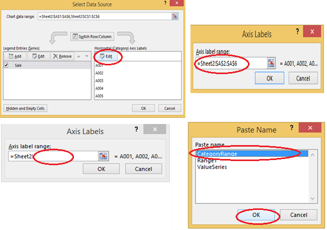
Step-3 Go to “Select Data” (Right click over chart and select from mini option), then select the Value series and click on edit. Now in Series Value box delete the range (Not sheet name) and replace with a defined name range of values by pressing F3 key.

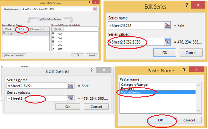
Step -4 Now Click on Edit button of Category and change the range with the defined range name of Categories and press OK.

 Now, whenever there is any addition or deletion of rows in dataset chart will change automatically.

End Notes:

In this article, we have discussed solution to a very common problem which a lot of Excel models suffer from. These methods will allow you to create dynamic ranges and use them in Excel charts and Pivots of your Excel models. These should enable you to automate your reports and model refreshes. As discussed, this outcome can also be achieved by using functions OFFSET and INDIRECT.

Have you faced any other common problems with your excel models? If yes, please feel free to share them here and we’ll try and solve them for you.

If you want to stay updated on latest analytics jobs, follow our job postings on twitter or like our Careers in Analytics page on Facebook

Sunil Ray 17 Apr 2015

I am a Business Analytics and Intelligence professional with deep experience in the Indian Insurance industry. I have worked for various multi-national Insurance companies in last 7 years.