How to avoid Over-fitting using Regularization?
Occam’s Razor, a problem solving principle states that
“Among competing hypotheses, the one with the fewest assumptions should be selected. Other, more complicated solutions may ultimately prove correct, but—in the absence of certainty—the fewer assumptions that are made, the better.”
Business Situation:
In the world of analytics, where we try to fit a curve to every pattern, Over-fitting is one of the biggest concerns. However, in general models are equipped enough to avoid over-fitting, but in general there is a manual intervention required to make sure the model does not consume more than enough attributes.
Let’s consider an example here, we have 10 students in a classroom. We intend to train a model based on their past score to predict their future score. There are 5 females and 5 males in the class. The average score of females is 60 whereas that of males is 80. The overall average of the class is 70.
Now, there are several ways to make the prediction:
- Predict the score as 70 for the entire class.
- Predict score of males = 80 and females = 60. This a simplistic model which might give a better estimate than the first one.
- Now let’s try to overkill the problem. We can use the roll number of students to make a prediction and say that every student will exactly score same marks as last time. Now, this is unlikely to be true and we have reached such granular level that we can go seriously wrong.
The first case here is called under fit, the second being an optimum fit and last being an over-fit.
Have a look at the following graphs,
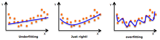
Image source: pingax.com
The trend in above graphs looks like a quadratic trend over independent variable X. A higher degree polynomial might have a very high accuracy on the train population but is expected to fail badly on test dataset. We will briefly touch up on various techniques we use to avoid over-fitting. And then focus on a special technique called Regularization.
Methods to avoid Over-fitting:
Following are the commonly used methodologies :
- Cross-Validation : Cross Validation in its simplest form is a one round validation, where we leave one sample as in-time validation and rest for training the model. But for keeping lower variance a higher fold cross validation is preferred.
- Early Stopping : Early stopping rules provide guidance as to how many iterations can be run before the learner begins to over-fit.
- Pruning : Pruning is used extensively while building CART models. It simply removes the nodes which add little predictive power for the problem in hand.
- Regularization : This is the technique we are going to discuss in more details. Simply put, it introduces a cost term for bringing in more features with the objective function. Hence, it tries to push the coefficients for many variables to zero and hence reduce cost term.
Regularization basics
A simple linear regression is an equation to estimate y, given a bunch of x. The equation looks something as follows :
y = a1x1 + a2x2 + a3x3 + a4x4 .......
In the above equation, a1, a2, a3 … are the coefficients and x1, x2, x3 .. are the independent variables. Given a data containing x and y, we estimate a1, a2 , a3 …based on an objective function. For a linear regression the objective function is as follows :
![]()
Now, this optimization might simply overfit the equation if x1 , x2 , x3 (independent variables ) are too many in numbers. Hence we introduce a new penalty term in our objective function to find the estimates of co-efficient. Following is the modification we make to the equation :
![]()
The new term in the equation is the sum of squares of the coefficients (except the bias term) multiplied by the parameter lambda. Lambda = 0 is a super over-fit scenario and Lambda = Infinity brings down the problem to just single mean estimation. Optimizing Lambda is the task we need to solve looking at the trade-off between the prediction accuracy of training sample and prediction accuracy of the hold out sample.
Understanding Regularization Mathematically
There are multiple ways to find the coefficients for a linear regression model. One of the widely used method is gradient descent. Gradient descent is an iterative method which takes some initial guess on coefficients and then tries to converge such that the objective function is minimized. Hence we work with partial derivatives on the coefficients. Without getting into much details of the derivation, here I will put down the final iteration equation :
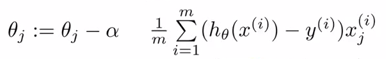 Here, theta are the estimates of the coefficients. Alpha is the learning parameter which will guide our estimates to convergence. Now let’s bring in our cost terms. After taking the derivative of coefficient square, it reduces down to a linear term. Following is the final iteration equation you get after embedding the penalty/cost term.
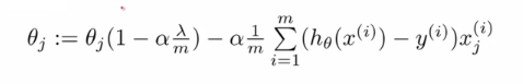
Now if you look carefully to the equation, the starting point of every theta iteration is slightly lesser than the previous value of theta. This is the only difference between the normal gradient descent and the gradient descent regularized. This tries to find converged value of theta which is as low as possible.
End Notes
In this article we got a general understanding of regularization. In reality the concept is much deeper than this. In few of the coming articles we will explain different types of regularization techniques i.e. L1 regularization, L2 regularization etc. Stay Tuned!
Did you find the article useful? Have you used regularization to avoid over-fit before? Share with us any such experiences. Do let us know your thoughts about this article in the box below.
If you like what you just read & want to continue your analytics learning, subscribe to our emails, follow us on twitter or like our facebook page.
Tavish Srivastava, co-founder and Chief Strategy Officer of Analytics Vidhya, is an IIT Madras graduate and a passionate data-science professional with 8+ years of diverse experience in markets including the US, India and Singapore, domains including Digital Acquisitions, Customer Servicing and Customer Management, and industry including Retail Banking, Credit Cards and Insurance. He is fascinated by the idea of artificial intelligence inspired by human intelligence and enjoys every discussion, theory or even movie related to this idea.


Hi Tavish Did you write the article about using L1 and L2 regularization? Thanks Rakesh
You are right Rakesh.
Hi, just want to point out for accuracy to reflect a real world scenario, you should have average score of boys be 60% and average score of girls be 80%. Peace!