Your Guide to Master Hypothesis Testing in Statistics
Introduction – the difference in mindset
I started my career as a MIS professional and then made my way into Business Intelligence (BI) followed by Business Analytics, Statistical modeling and more recently machine learning. Each of these transition has required me to do a change in mind set on how to look at the data.
But, one instance sticks out in all these transitions. This was when I was working as a BI professional creating management dashboards and reports. Due to some internal structural changes in the Organization I was working with, our team had to start reporting to a team of Business Analysts (BA). At that time, I had very little appreciation of what is Business analytics and how is it different from BI.
So, as part of my daily responsibilities, I prepared my management dashboard in the morning and wrote a commentary on it. I compared the sales of first week of the current month to sales of previous month and same month last year to show an improvement in business. It looked something like this:
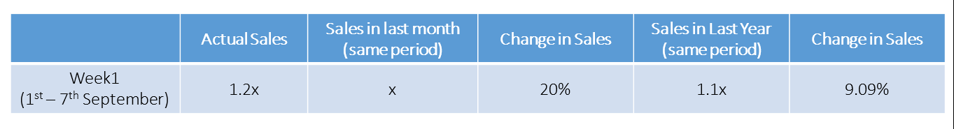
In my commentary, I ended up writing that sales are better than last year and last month and applauded some of the new initiatives the Sales team had taken recently. I was thinking this was good work to show to my new manager. Little did I know, what was in store!
When I showed the report to my new manager applauding the sales team, he asked why do I think this uplift is just not random variation in data? I had very little Statistics background at this time and I could not appreciate his stand. I thought we were talking 2 different language. My previous manager would have jumped over this report and would have dropped a note to Senior Management himself! And here was my new manager asking me to hold my commentary.
In today’s article, I will explain hypothesis testing and reading statistical significance to differentiate signal from the noise in data – exactly what my new manager wanted me to do!
P.S. This might seem like a lengthy article, but would be one of the most useful one, if you follow through.
A case study:
Let us say that average marks in mathematics of class 8th students of ABC School is 85. On the other hand, if we randomly select 30 students and calculate their average score, their average comes to be 95. What can be concluded from this experiment? It’s simple. Here are the conclusions:
- These 30 students are different from ABC School’s class 8th students, hence their average score is better i.e behavior of these randomly selected 30 students sample is different from the population (all ABC School’s class 8th students) or these are two different population.
- There is no difference at all. The result is due to random chance only i.e. we found the average value of 85. It could have been higher / lower than 85 since there are students having average score less or more than 85.
How should we decide which explanation is correct? There are various methods to help you to decide this. Here are some options:
- Increase sample size
- Test for another samples
- Calculate random chance probability
The first two methods require more time & budget. Hence, aren’t desirable when time or budget are constraints.
So, in such cases, a convenient method is to calculate the random chance probability for that sample i.e. what is the probability that sample would have average score of 95?. It will help you to draw a conclusion from the given two hypothesis given above.
Now the question is, “How should we calculate the random chance probability?“.
To answer it, we should first review the basic understanding of statistics.
Basics of Statistics
1. Z-Value/ Table/ p value: Z value is a measure of standard deviation i.e. how many standard deviation away from mean is the observed value. For example, the value of z value = +1.8 can be interpreted as the observed value is +1.8 standard deviations away from the mean. P-values are probabilities. Both these statistics terms are associated with the standard normal distribution. You can look at the p-values associated with each z-value in Z-table. Below is the formula to calculate z value: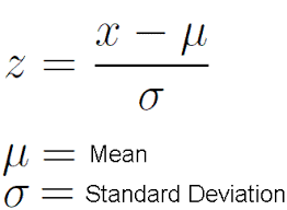
Here X is the point on the curve, μ is mean of the population and σ is standard deviation of population.
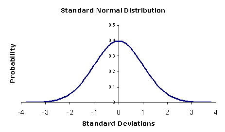 As I discussed, these methods always work with normal distribution (shown above) only, not with other distributions. In case, the population distribution is not normal, we’d resort to Central Limit Theorem.
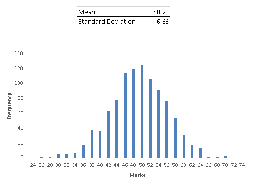
2. Central Limit Theorem: This is an important theorem in statistics. Without going into definitions, I’ll explain it using an example . Let’s look at the case below. Here, we have a data of 1000 students of 10th standard with their total marks. Following are the derived key metrics of this population:
And, frequency distribution of marks is:
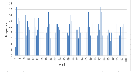 Is this some kind of distribution you can recall? Probably not. These marks have been randomly distributed to all the students.
Now, let’s take a sample of 40 students from this population. So, how many samples can we take from this population? We can take 25 samples(1000/40 = 25). Can you say that every sample will have the same average marks as population has (48.4)? Ideally, it is desirable but practically every sample is unlikely to have the same average.
Here we have taken 1000 samples of 40 students (randomly sample generated in excel). Let’s look at the frequency distribution of these sample averages of thousands samples and other statistical metrics:
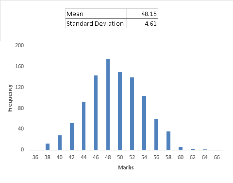
Does this distribution looks like the one we studied above? Yes, this table is also normally distributed. For better understanding, you can download this file from here and while doing this exercise you’ll come across the findings stated below:
1. Mean of sample means (1000 sample means) is very close to population mean
3. The distribution of sample means is normal regardless of the distribution of the actual population. This is known as Central Limit theorem. This can be very powerful. In our initial example of ABC School students, we compared the sample mean and population mean. Precisely, we looked at the distribution of sample mean and found out the distance between population mean and the sample mean. In such cases, you can always use a normal distribution without worrying about the population distribution.
You can calculate the standard deviation and mean based on above findings and calculate z-score and p-value. Here random chance probability will help you to accept one of discussed conclusions from ABC School’s example (stated above). But, to satisfy the CLT theorem, sample size must be sufficient (>=30).
Now, let’s say we have calculated the random chance probability. It comes out to be 40%, then should I go with first conclusion or other one ? Here the “Significance Level” will help us to decide.
What is Significance Level?
We have taken an assumption that probability of sample mean 95 is 40%, which is high i.e. more likely that we can say that there is a greater chance that this has occurred due to randomness and not due to behavior difference.
Had the probability been 7%, it would have been a no-brainer to infer that it is not due to randomness. There may be some behavior difference because probability is relatively low which means high probability leads to acceptance of randomness and low probability leads to behavior difference.
Now, how do we decide what is high probability and what is low probability?
To be honest, it is quite subjective in nature. There could be some business scenarios where 90% is considered to be high probability and in other scenarios could be 99%. In general, across all domains, cut off of 5% is accepted. This 5% is called Significance Level also known as alpha level (symbolized as α). It means that if random chance probability is less than 5% then we can conclude that there is difference in behavior of two different population. (1- Significance level) is also known as Confidence Level i.e. we can say that I am 95% confident that it is not driven by randomness.
Till now, we looked at the tools to test a hypothesis, whether sample mean is different from population or it is due to random chance. Now, let’s look at the steps to perform a hypothesis test and post that we will go through it using an example.
What are the steps to perform Hypothesis Testing?
- Set up Hypothesis (NULL and Alternate): In ABC School example, we actually tested a hypothesis. The hypothesis, we are testing was the difference between sample and population mean was due to a random chance. It is called as “NULL Hypothesis” i.e. there is no difference between sample and population. The symbol for the null hypothesis is ‘H0’. Keep in mind that, the only reason we are testing the null hypothesis is because we think it is wrong. We state what we think is wrong about the null hypothesis in an Alternative Hypothesis. For the ABC School example, alternate hypothesis is, there is a significant difference in behavior of sample and population. The symbol for the alternative hypothesis is ‘H1’. In a courtroom, since the defendant is assumed to be innocent (this is the null hypothesis so to speak), the burden is on a prosecutor to conduct a trial to show evidence that the defendant is not innocent. In a similar way, we assume the null hypothesis is true, placing the burden on the researcher to conduct a study to show evidence that the null hypothesis is unlikely to be true.
- Set the Criteria for decision: To set the criteria for a decision, we state the level of significance for a test. It could 5%, 1% or 0.5%. Based on the level of significance, we make a decision to accept the Null or Alternate hypothesis. There could be 0.03 probability which accepts Null hypothesis on 1% level of significance but rejects Null hypothesis on 5% of significance. It is based on business requirements.
- Compute the random chance of probability: Random chance probability/ Test statistic helps to determine the likelihood. Higher probability has higher likelihood and enough evidence to accept the Null hypothesis.
- Make Decision: Here, we compare p value with predefined significance level and if it is less than significance level, we reject Null hypothesis else we accept it. While making a decision to retain or reject the null hypothesis, we might go wrong because we are observing a sample and not an entire population. There are four decision alternatives regarding the truth and falsity of the decision we make about a null hypothesis:
1. The decision to retain the null hypothesis could be correct.
2. The decision to retain the null hypothesis could be incorrect, it is know as Type II error.
3. The decision to reject the null hypothesis could be correct.
4. The decision to reject the null hypothesis could be incorrect, it is known as Type I error.
Example
Blood glucose levels for obese patients have a mean of 100 with a standard deviation of 15. A researcher thinks that a diet high in raw cornstarch will have a positive effect on blood glucose levels. A sample of 36 patients who have tried the raw cornstarch diet have a mean glucose level of 108. Test the hypothesis that the raw cornstarch had an effect or not.
Solution:- Follow the above discussed steps to test this hypothesis:
Step-1: State the hypotheses. The population mean is 100.
H0: μ= 100
H1: μ > 100
Step-2: Set up the significance level. It is not given in the problem so let’s assume it as 5% (0.05).
Step-3: Compute the random chance probability using z score and z-table.
For this set of data: z= (108-100) / (15/√36)=3.20
You can look at the probability by looking at z- table and p-value associated with 3.20 is 0.9993 i.e. probability of having value less than 108 is 0.9993 and more than or equals to 108 is (1-0.9993)=0.0007.
Step-4: It is less than 0.05 so we will reject the Null hypothesis i.e. there is raw cornstarch effect.
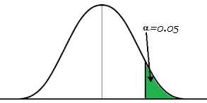
Note: Setting significance level can also be done using z-value known as critical value. Find out the z- value of 5% probability and it is 1.65 (positive or negative, in any direction). Now we can compare calculated z-value with critical value to make a decision.
Directional/ Non Directional Hypothesis Testing
In previous example, our Null hypothesis was, there is no difference i.e. mean is 100 and alternate hypothesis was sample mean is greater than 100. But, we could also set an alternate hypothesis as sample mean is not equals to 100. This becomes important when we do reject the Null hypothesis, should we go with which alternate hypothesis:
- Sample mean is greater than 100
- Sample mean is not equals to 100 i.e. there is a difference
Here, the question is “Which alternate hypothesis is more suitable?”. There are certain points which will help you to decide which alternate hypothesis is suitable.
- You are not interested in testing sample mean lower than 100, you only want to test the greater value
- You have strong believe that Impact of raw cornstarch is greater
In above two cases, we will go with One tail test. In one tail test, our alternate hypothesis is greater or less than the observed mean so it is also known as Directional Hypothesis test. On the other hand, if you don’t know whether the impact of test is greater or lower then we go with Two tail test also known as Non Directional Hypothesis test.
Let’s say one of research organization is coming up with new method of teaching. They want to test the impact of this method. But, they are not aware that it has positive or negative impact. In such cases, we should go with two tailed test.
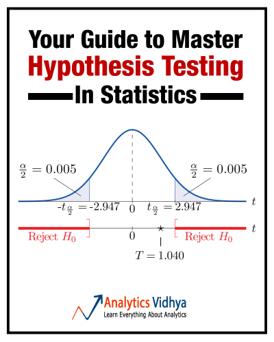
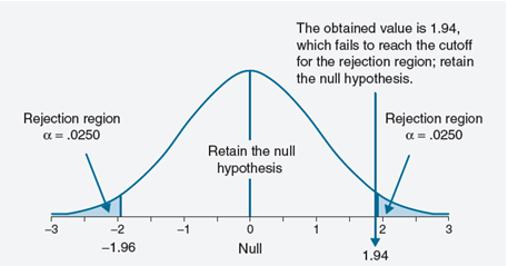
In one tail test, we reject the Null hypothesis if the sample mean is either positive or negative extreme any one of them. But, in case of two tail test we can reject the Null hypothesis in any direction (positive or negative).
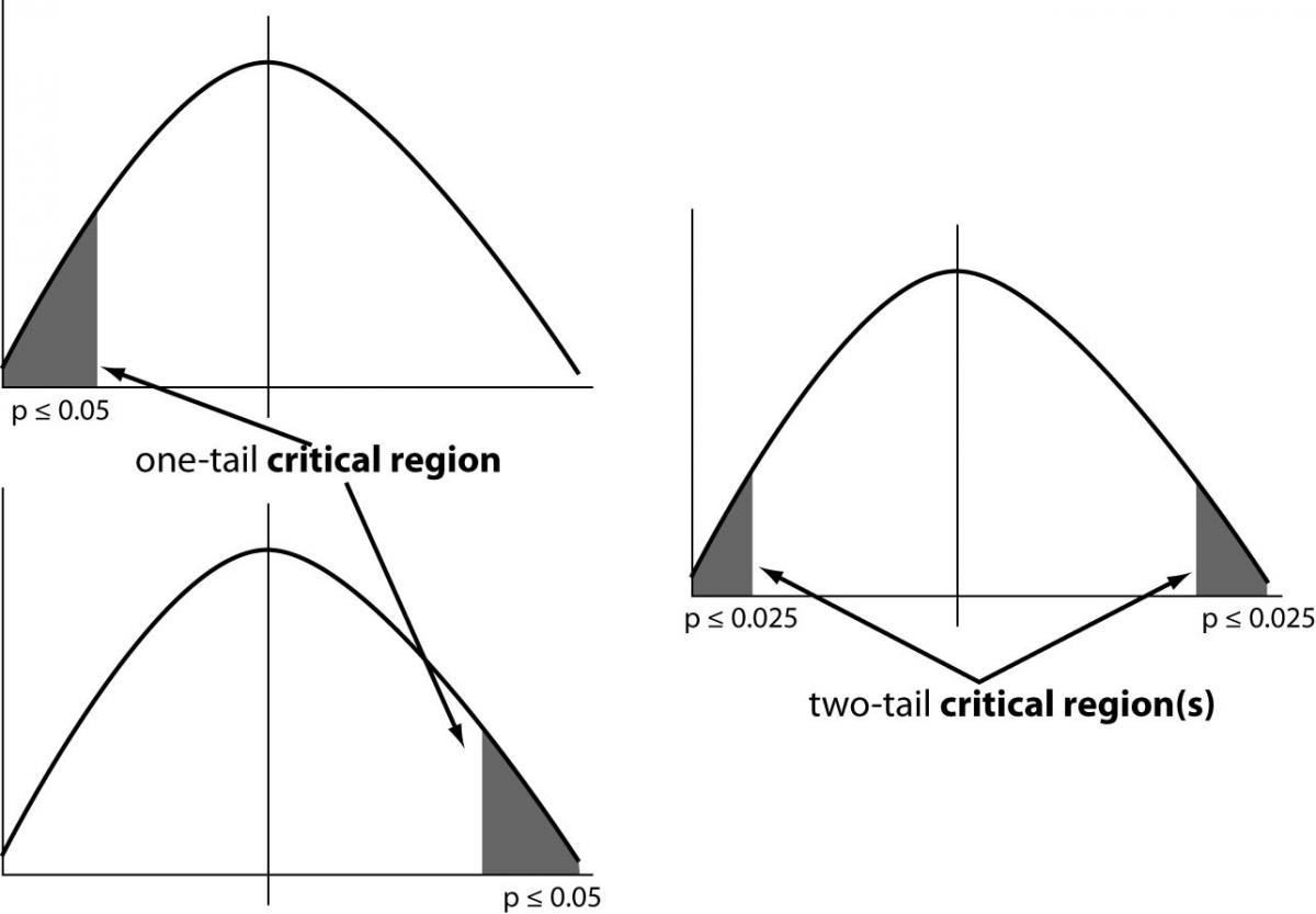
Look at the image above. Two-tailed test allots half of your alpha to testing the statistical significance in one direction and half of your alpha in the other direction. This means that .025 is in each tail of the distribution of your test statistic. Why are we saying 0.025 on both side because normal distribution is symmetric. Now we come to a conclusion that Rejection criteria for Null hypothesis in two tailed test is 0.025 and it is lower than 0.05 i.e. two tail test has more strict criteria to reject the Null Hypothesis.
Example
Templer and Tomeo (2002) reported that the population mean score on the quantitative portion of the Graduate Record Examination (GRE) General Test for students taking the exam between 1994 and 1997 was 558 ± 139 (μ ± σ). Suppose we select a sample of 100 participants (n = 100). We record a sample mean equal to 585 (M = 585). Compute the p-value t0 check whether or not we will retain the null hypothesis (μ = 558) at 0.05 level of significance (α = .05).
Solution:
Step-1: State the hypotheses. The population mean is 558.
H0: μ= 558
H1: μ ≠ 558 (two tail test)
Step-2: Set up the significance level. As stated in the question, it as 5% (0.05). In a non-directional two-tailed test, we divide the alpha value in half so that an equal proportion of area is placed in the upper and lower tail. So, the significance level on either side is calculated as: α/2 = 0.025. and z score associated with this (1-0.025=0.975) is 1.96. As this is a two-tailed test, z-score(observed) which is less than -1.96 or greater than 1.96 is a evidence to reject the Null hypothesis.
Step-3: Compute the random chance probability or z score
For this set of data: z= (585-558) / (139/√100)=1.94
You can look at the probability by looking at z- table and p-value associated with 1.94 is 0.9738 i.e. probability of having value less than 585 is 0.9738 and more than or equals to 585 is (1-0.9738)=0.03
Step-4: Here, to make a decision, we compare the obtained z value to the critical values (+/- 1.96). We reject the null hypothesis if the obtained value exceeds a critical values. Here obtained value (Zobt= 1.94) is less than the critical value. It does not fall in the rejection region. The decision is to retain the null hypothesis.
End Notes
In this article, we have looked at the complete process of undertaking hypothesis testing during predictive modeling. Initially, we looked at the concept of hypothesis followed by the types of hypothesis and way to validate hypothesis to make an informed decision. We also have also looked at important concepts of hypothesis testing like Z-value, Z-table, P-value, Central Limit theorem.
As mentioned in the introduction, this was one of the most difficult change in mindset for me when I read this first time. But it was also one of the most helpful and significant change. I can easily say that this change started me to think like a predictive modeler.
In next article, we will look at the what-if scenarios with hypothesis testing like:
- If sample size is less than 30 (Not satisfy CLT)
- Compare two sample rather than sample and population
- If we don’t know the population standard deviation
- p-values and Z-scores in the Big Data age
Did you find this article helpful? Please share your opinions / thoughts in the comments section below.
If you like what you just read & want to continue your analytics learning, subscribe to our emails, follow us on twitter or like our facebook page.
I am a Business Analytics and Intelligence professional with deep experience in the Indian Insurance industry. I have worked for various multi-national Insurance companies in last 7 years.


Thanks for posting this article - An excellent read
Nice article.
Hi Sunil, Very nice article. Keep up the good work! Regards Gaurav
excellent analysis
Hey Sunil, I think this article was the best because you start with a challenge in work that every person may face
Great Article Sunil. This was helpful. Keep it coming. Thanks, Kishore
It was really helpful.Its great to see how you give real life examples from your work.Want to see more statistics in your blog. Cheers!!
Hi Sunil, Thanks for the excellent article. I wanted to understand this from long time however thickness of stat books kept me away. You did great job in keeping a story along with fundamental of stats. Cheers
good job!!!!
Hi All, Thanks for the comment … Regards, Sunil
Very insightful!! I have one question So does it means that if random chance probability is less than 5 % then there is difference in the behavior of two population and it is due to randomness?
If the p-value (random chance probability) is less than 5% then yes very likely you are correct in your conclusion that there is systematic difference between the two groups and the difference is NOT due to random chance. Or you can also say that you are 95% confident in your conclusion.
Hi Shilpi, Suppose I have observed data with me..lets say I have 48 files comprising of 24 male gender files and 24 female gender files which will be represented to a board of members of the firm who will evaluate these files based on their performance for promotion. Lets say out of 24 males, 18 were promoted and out of 24 females only 11 were promoted to higher ranks. so there is a 30% observed difference in promotion of males and females. based on our observed finding I know wants to test the hypothesis if there is any relationship between promotion and gender? Is their any bias towards males than females when it comes to promotion of employees? I start by saying that lets assume there is no relationship between gender and promotion i.e. there is no effect in the population. So I initially assume my null hypothesis to be true. The other hypothesis which is my alternative hypothesis says that there is an effect in the population i.e. there is a relationship between gender and promotion for which i want to conduct hypothesis testing. By simulating this process for 100 times, lets say that it happened on less than 5% chances(Only on less than 5 instances in 100) that such a large difference of 30% occurred in gender promotion which points out that this observed difference of 30% in our original data didn't happened by chance but is a case of bias towards the gender when it comes to their promotion..so p-value is the probability of occurrence of an effect in the population assuming null hypothesis to be true which in this case is less than 5%(very rare in my simulations that such a high value will occur)..Hope it gets clear!
Easy to understand and concise. I had this learning from my course I took from Jigsaw Academy but had lost some touch. Thanks for putting across this very important article.
That's by far the best content I've ever read regarding hypothesis testing. Thankyou Sunil and team!! Looking forward to reading more of your articles.
Nice job! Where do we find the next article?
Hi, Nice post! I am interested of how you answered your boss? What was the solution to the "signal or noise" original problem?
Thank you for this article !
Thanks for such great Article, you explained this concept very easily Regard
Great read, although some images are missing. Please will you make these images available again.
A fantastic read...Great job.
You can look at the probability by looking at z- table and p-value associated with 3.20 is 0.9993 i.e. probability of having value less than 108 is 0.9993 and more than or equals to 108 is (1-0.9993)=0.0007. Can anyone explain how we inferred that 0.9993 is probability of having value less than 108. It can be probability of greater than 108 also ?
Great breakdown! Thank you.
"You can look at the probability by looking at z- table and p-value associated with 3.20 is 0.9993 i.e. probability of having value less than 108 is 0.9993 and more than or equals to 108 is (1-0.9993)=0.0007. Step-4: It is less than 0.05 so we will reject the Null hypothesis i.e. there is raw cornstarch effect."-copied from above article. probability of having value less than 108 is 0.9993 means its supporting to null hypo with high which mean value is 100. please clarify I am not getting this point. Thanks
Great article, it is really helpful for beginners in research ie data analysis. But please somebody tell me that wether we can use t-test for a sample greater than 30 to compare two groups for cause and effect relationship. The effect of matching/mismatching of teaching and learning styles on academic achievement where the sample is greater than 300.
Thanks for this nice POST and making the concept simple to understand
Thanks for the share, learnt big time
Hi, I am failing to understand the relation between the null hypothesis and the inference for the 1st example with the blood glucose level.. The Null and alternate hypothesis are set for 100 and > 100, however the inference talks about less than 108 vs greater than 108. Can some one help me relate the hypothesis to the inference? Thanks, Siva
Hi Sunil, Nice article, you explain it nicely with simple worlds, and nice charts, I like it :) I want to mention that the examples are based on the assumption that the population distribution is normal, this assumption also should be checked. Also, I want to mention that in the example we know the population's standard deviation, usually, we don't know the population's standard deviation, and we need to estimate the value based on the sample. in this case, we should use the t distribution instead of the normal distribution (z)
today is my exam on bio-statistics, and i am not ready..... but suddenly i viewed this article. it helps me a lot..... thank you so much -Samson- fr: Philippines
[…] mean is right around zero, with a standard deviation of 7.3. You’ll see the formula broken out here, as we snag the z-score for this value and produce -0.328: our tanking rookies barely differ from […]
Good article to explain clearly the CLT and Null Hypothesis setting with Confidence Levels... Good to refresh my knowledge on statistical analysis...
This was so good, thanks you a lot, so helpfull