Quick Guide to learn Statistics for R Users (with Titanic Data Set)
Introduction
People are keen to pursue their career as a data scientist. And why shouldn’t they be? After all, this comes with a pride of holding the sexiest job of this century. But, in order to become one, you must master ‘statistics’ in great depth.
Statistics lies at the heart of data science. Think of statistics as the first brick laid to build a monument. You can’t build great monuments until you place a strong foundation. Experts say, ‘If you struggle with deciphering the statistical coefficients , you’d have tough time ahead in data science’.
Don’t worry! I shall help you decipher some of these statistical mysteries in this post. I will use R as my tool to perform the calculations, but you can choose any tool of your convenience.
What will you learn from this article?
Statistics has two arms: Descriptive Statistics and Inferential Statistics. Both arms deal with analyzing data, but with different objectives. Descriptive statistics help us describe large data sets, while inferential statistics help us draw inference about population from a sample of this population.
I haven’t explained these concepts in detail as they are already discussed in understanding statistics. I’ve laid emphasis on the practical aspect of statistics rather than theoretical. Hence, I strongly recommend to refer to this article to maximum benefit from what is described here.
I’ve considered titanic data set for practical purpose.
Note: This article is best suited for beginners and intermediates in data science, who are facing difficulty in dealing with statistical concepts.
Descriptive Statistics
‘Descriptive’, the term originated from the word ‘describe’ means explain. It is used to explain the characteristics of a data set using measures such as mean, mode, median, variance etc. These measures summarize data and help you draw meaningful patterns.
Descriptive Statistics can further be divided into two parts:
- Measures of Central Tendency; and
- Measures of Spread.
Let’s understand these measures one by one:
Measure of Central Tendency
Mean (Average): It is calculated as the sum of all values in a data set / number(count) of values. It can be used with both discrete and continuous variables, but, it is often used with continuous variables.
Mean = Sum of all Observations / No. of Observations
A major disadvantage of using mean is, it is highly affected by outliers. Also, mean cannot be used while dealing with categorical (nominal) values and skewed distributions. In such cases, we make use of mode/ median.
Let’s find, the average value of Fare (variable in data set) charged to board Titanic Ship.
#set working directory
setwd("C:/Users/manish/Desktop/RData")
#load the data set
train <- read.csv("C:/Users/manish/Desktop/Titanic/train1.csv", stringsAsFactors = FALSE, header = T)

#find the average(mean) Fare
mean(train$Fare)
[1] 32.20421
Interpretation: On an average, passengers have paid $32 to board the titanic.
Mode: Think of ‘Mode’ as ‘repeat’. Mode is nothing but the value that has been repeated the maximum number of times in a data set. In other words, it is the value of a observation having highest frequency.
R does not have any inbuilt function to find out Mode. However, it does have a mode() function which returns the type or storage mode of an object instead. Let’s see how to find out the age with highest frequency.
#using inbuild mode function
mode(train$Age)
[1] "numeric"
#using a simple method
actual_mode <- table(train$Age)    #creates a table of all age groups
#view the output of actual_mode
actual_mode                        #let's treat the age values here as names
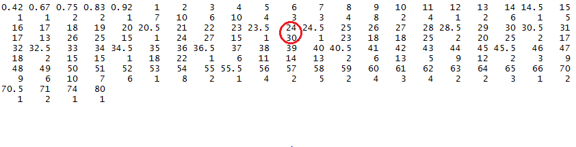
#find the most frequent value using max
names(actual_mode)[actual_mode == max(actual_mode)]
[1] "24"
Interpretation: Most common age among passengers on Titanic was 24 years. As you can see, there were 30 passengers on board who are 24 years old (highest among all).
Median: Think of ‘Median’ as the mid point of all values in data set. Median divides the data set into two equal halves such that one half is less than median and the other greater.
Median values are less affected by outliers. Also, it is based on all observations and easy to compute. Let’s compute the median of Fare.
#find out the median
median(train$Fare)
[1] 14.4542
Interpretation: The mid value of Fare variable is $14.45. This means $14.45 divides the data into two halves. If you compute its range, along with this statistic, you’ll find the this variable is highly skewed (don’t worry, if you don’t understand – we will discuss these terms shortly).
Measure of Spread
Measure of spread represents the variability in a sample or population. Using this measure, you get to know the amount of variation among observations, which can later be treated using suitable measures. Often, people relate measure of spread with box plot summary. I’ve discussed it as well.
Range: It represents the complete extent of data. It shows the lowest value and the highest value in a set of observation. We can calculate range using this simple function:
#calculate range
range(train$Fare)
[1] 0.0000 512.3292
Quartile: It divides the data set into 4 equal parts using Q1 (First Quartile), Q2 (Second Quartile) and Q3 (Third Quartile). Let’s understand it using an example, assume we have a numerical variable having values from 1 to 100. Here, value for Q1 would be 25 (value at 25th percentile), value for Q2 would be 50 (value at 50th percentile i.e. median) and value for Q3 would be 75 (value at 75th percentile).
Quartiles are well understood when used with box plots. Box Plots is a five number summary which represents Minimum, Maximum, Q1, Q2 and Q3. Let’s find out.
#find boxplot
boxplot(train$Age ~ train$Pclass, xlab = "Class", ylab = "Age", col = c("red"))
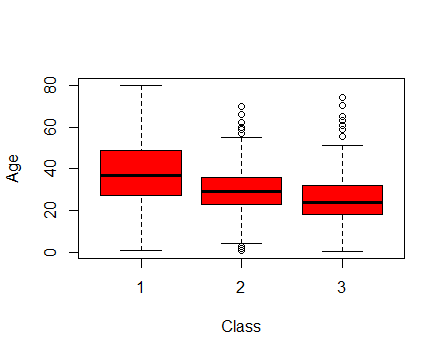
Interpretation: After analyzing this box plot of Class and Age, we can infer that the median value of Class 1 passengers is higher than that of Class 2 and Class 3. It means Class 2 and Class 3 had younger passengers than Class 1. Infact, class 3 had the youngest age group of passengers. The tiny circles outside the range of Class 2 and Class 3 represents the outlier values.
Variance and Standard Deviation: Variance and Standard Deviations are closely related. In simple words:
SQRT(variance) = Standard Deviation
Variance is the average of squared difference from mean. In R, you don’t need to get into mathematics of these measures since we have inbuilt functions to calculate these values. Let’s find out the variance & standard deviation for Fare variable.
#variance of fare
var(train$Fare)
[1] 2469.437

#Standard Deviation of Fare
sqrt(var(train$Fare))
[1] 49.69343
Distributions: Simply put, distribution refers to the way population is spread on a particular dimension. This article helps you understand various terms used to describe shapes of distribution.
Let’s look at the distribution of Fare using a bar chart:
#create bar chart of Fare
hist(train$Fare, main = "Fare Per Person", xlab = "Fare", col = "grey", breaks = 40,
     xlim = c(0,300))
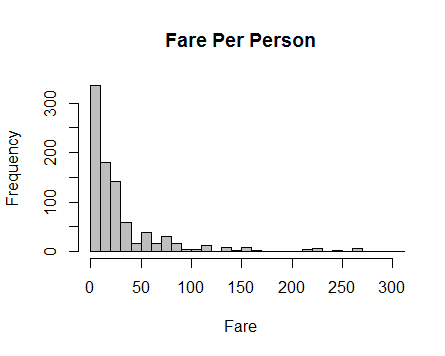
Question: How is this distribution skewed? Positive or Negative?
Some modeling techniques (like regressions) make an assumption about the underlying distributions of the population. In case your population does not fulfill them, you may need to make some transformations to improve the results of your models.
Live Update: Register Now in ‘The D Hack’ and win Amazon Vouchers worth Rs. 20,000 (~$300)
Inferential Statistics
These statistical measures is used to make inferences about larger population from sample data. In other words, we can say that inferential statistical measures help us to make judgement for population on the basis of insights generated from sample. Let’s find out the inference which we can draw from titanic data set:
Hypothesis Testing: You can quickly revise your basics of hypothesis testing with this guide to master hypothesis in statistics.
Let’s say, we want to check the significance of variable Pclass for hypothesis testing . Let’s assume that upper class( Class 1) has better chances of survival than its population.
To verify our assumption, let’s use z-test and see, if passengers of upper class have better survival rate than its population.
Hº: There is no significant difference in the chances of survival of upper and lower class
H1: There is a better chance of survival for upper class passengers
#calculate z test
#create a new data frame for upper class passengers
new_data <- subset(train, train$PClass == 1)
#function for z test
z.test2 = function(a, b, n){
 sample_mean = mean(a)
 pop_mean = mean(b)
 c = nrow(n)
 var_b = var(b)
 zeta = (sample_mean - pop_mean) / (sqrt(var_b/c))
 return(zeta)
}

#call function
z.test2(new_data$Survived, train$Survived, new_data)
[1] 7.423828
Finally, our z value comes out to be 7.42 which affirms our suggestion that upper class has better chances of survial than its population. High z value denotes that p value will be very low. Similarly, you can check the significance of other variables.
Chi-Square Test: This test is used to derive the statistical significance of relationship between the variables. Also, it tests whether the evidence in the sample is strong enough to generalize that the relationship for a larger population as well. Chi-square is based on the difference between the expected and observed frequencies in one or more categories in the two-way table. It returns probability for the computed chi-square distribution with the degree of freedom.
Probability of 0: It indicates that both categorical variable are dependent
Probability of 1: It shows that both variables are independent.
Probability less than 0.05: It indicates that the relationship between the variables is significant at 95% confidence.
R has a inbuilt function for chi-square test. Let’s now check this test in our data set :
#chi-square test between Survived, Sex, Pclass chisq.test(train$Survived, train$Sex)#another method of chi-square test summary(table(train$Survived,train$Pclass))
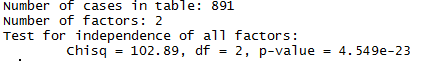
Interpretation: Since their p values < 0.05, we can infer, Sex and Pclass are highly significant variables and must be included in our final modeling stage. But, this is just the beginning. As you continue checking for other variables, you’ll find other significant variables as well. Don’t forget feature engineering. It can totally change your game.
Correlation: Correlation determines the level of association between two variables. You can quickly revise your basics from 7 most asked questions on correlation.
Let’s find out the level of association in the variables of this data set. It is considered to be a good practice to check out scatter plot among the variables to find access their correlation. For example: Let’s plot Fare vs Age.
plot(train$Fare, train$Age, xlab = 'Fare', ylab = 'Age')
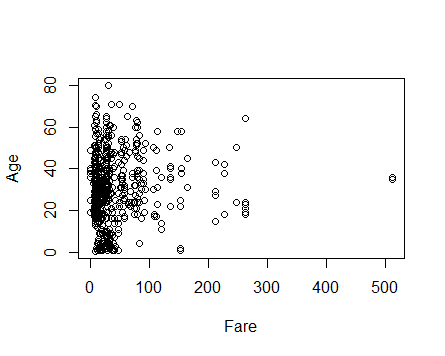
Can you see any correlation in these variables? I certainly don’t because there is no pattern (positive or negative) which can suggest us of their correlation. Let’s confirm our result now:
#pearson correlation test
cor.test(train$Age, train$Fare, method = 'pearson')
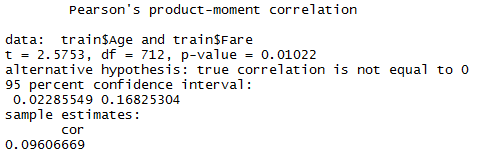
Interpretation: Just like we assumed, this statistics further corroborates our assumption that there exist very low association between fare and age. This test confirm the strength of correlation is meager 9.6%. Similarly, you can find association among other variables. If you find any highly correlated variable, you can also drop of these variables from your final model as it won’t add lot of new information in the model.
Regression: Regression is used to access the level of relationship between two or more variables. It is driven by predictor (independent variable) and response(dependent variable). For a quick refresher, I suggest you to read 7 types of regression techniques.
Here are few things you must acknowledge before proceeding for regression:
- I haven’t performed any sort of feature engineering. However, I strongly suggest you to do so.
- You’ll see, the performance of my regression model wouldn’t be effective because I’ve left out some significant variables which can be obtained after feature engineering.
- Since our dependent variable is categorical, we’ll use logistic regression.
Dependent Variable(Y): Survival
Independent Variable(X): Pclass, Age, Sex, SibSp, Parch, Fare, Embarked
#Regression model
fit <- glm(Survived ~ Age + Pclass + Sex + SibSp + Parch + Fare + Embarked + Cabin,                     data = train, family = binomial(link = 'logit'))
summary(fit)
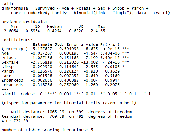
Interpretation: As expected, the output is disappointing. AIC criterion, which measures the goodness of fit is extremely high(727.39). Lower the AIC value, better will be the model. You can read more about AIC here.
There are two things which we learn here:
- To build any model, choose the right algorithm according to its variables.
- Never rely on available variables in the data set, learn to read between the ‘variables’. You may find highly significant knowledge buried there.
End Notes
When I started with statistics, I knew the theory of these measures, but I was not clear about practical uses of these measures and how they help. In this article, I’ve illustrated the used of statistical concepts using a practice problem (titanic).
Some of the statistical measure aren’t so useful when used in isolation. For example, Mean. You know the mean of one variable. What do you do now? Nothing, until you compare it with other variables. Hence, you should be sure when to use which measure. I found a quick guide on, when to use which statistical measure? , published by California State University. This can surely be of your help.
If there is any further knowledge which you think can be added to this article, please feel free to share it in the comments section below.


Hi Manish.... Excellent !!! I find data analytics so interesting that I have chosen this field of study inorder to shift my career into business analytics. Through this article of yours, you have helped me understand the basics so well that I have gained immense confidence that I can do justice to what I have taken up. Kindly consider this message from me as a "token of appreciation" and inspire us through your generous help. All the best for all your endeavours !!!
Thank You Thirumal for your kind words!
Just wanted to add..... Amongest all the good work in the article, the point that stands out for me is the way it has been kept simple alongwith the sentence URLs for references. As many feel, I too want to state that "Analytics Vidya" on the whole is doing an excellent work....!!! Rockiing !!! Thank you guys!!!
Hi I wanted to switch my careet to BI once I finish my MSIS degree. I am going to learn statistics as one of a course for program. I also have worked on Cognos, BI reports and tableau. What else should I learn in order to transition my career in BI? Also just learning and not having hands on will impact my career ?
Wonderful article! So far I've been to this site twice and each time have come away with a wealth of knowledge! Keep up the good work!
Thanks Kem
Hi Manish, Thanks for the well described article. It cleared my concepts on statistics. very helpful when described with example. R has an inbuilt function to directly calculate standard deviation of a variable. just call : sd(var_name)
Thank Himansu P.S - I didn't know about sd(var_name), this will help me write one command less. Keep sharing knowledge.
Excellent Article, good coverage of variety of statistics/methods within this article,
Thank you Ramdas
Great post and sources Manish. Bookmarked and shared!
Thanks George!
Good article, I just finished Statistics Unplugged (which I respect for any newbies) and I really enjoyed the article. I look forward to working through the examples in R. Thanks!
Thanks MIke !
Hi aov stands analysis of variance in R ?? In such case only F test is used to check any significant difference among variables in anova But how Chi square test is used ?? Please direct me in case am wrong Thanks Raju
Hi Raj Thanks for highlighting this error. I should have noticed it. My Bad! Chi-square test is used to check the dependence of categorical variables whereas Analysis of variance is used to compare means between two samples where the variance in means is determined by treatment mean square. And that's why I've considered Chi-square with Sex, Survived and Pclass to check for significance.
Well explained. I just completed my data analytics course but still dont understand some statistical explanation. Still requested help to understand. Manish make my job simple. Easy to understand and follow. Bookmarked and share with my friends. Great source of learning. Thanks Manish.
Hi! Thanks for sharing! I have a question about checking the significance of variable Pclass for hypothesis testing. This article used Z-test to calculate the p-value, We know that one of the assumptions of Z test is that the sample distribute normally, but the survival rate is a categorical feature, and does not distribute normally. Is it appropriate to calculate standard deviation in this case?? Again, thanks for your sharing^^!
Hi Manesh, Good article thanks. Would the median in the example with numbers 1... 100 not be the value of 50.5? As in we have an even number of data points & therefore we would need to take the 50th & 51st point & get the average. Similarly or Q1 & Q3 (at 25.5 & 75.5 resp.). thanks John
Great article man, thank you! By the way, in the below code please change "Class1" to "Pclass" #create a new data frame for upper class passengers new_data <- subset(train, train$Class1 == 1) Thanks again mate! (^_^)
thank you for brilliant information I think it is good idea to put a print icon to print articles best regards
Ability to explain complex matter in simple words is required -command on subject. I feel team Analytics is having this command and presenting text in very motivating manner. Technical terms with links for deatil is really helpful. keep updating. thanks.