Getting started with Machine Learning in MS Excel using XLMiner

Introduction

Machine Learning is nothing but building a ‘machine’ which ‘learns’ from its experience. And, becomes better with experience – just like humans. We also learn from our experiences. Right ? Companies like Google, Facebook, Microsoft are using machine learning techniques at a larger scale.

However, one common mis-conception people have is that they need to learn coding to start machine learning. While coding becomes necessary for any one who is doing machine learning seriosuly, but not to start it. You can look at GUI driven tool like Weka or even Excel to start with Machine Learning.

Here, I’ll introduce you to a simpler way to get started with Machine Learning.

Do you find coding hard to understand?

Machine Learning requires powerful coding / algorithmic skills. And that’s why, people with computer science degree find it relatively easier to succeed in machine learning domain.

But, the scenario has changed. Though, you can’t escape coding completely, you can still get started with machine learning. Once you get started, you can later brush up your coding skills.

The good news is, now you can start machine learning using Microsoft Excel. Yes! you heard it right.

Frontline Solvers has introduced ‘XLMINER DATA MINING‘ add-in for MS Excel. It is an easy to use, made for professionals tool for data visualization, forecasting and data mining.  You’d find it easy to use if:

1. You’ve worked on MS Excel in past
2. You’ve working experience of SPSS

Also Read: Simple Yet Powerful Tricks To Analyze Data in Excel

What are the tasks XLMiner can do  ?

I knew this was coming. Well! XLMiner can do lot of things which you do in R, Python or Julia. That too, without writing a piece of code. It offers a great deal in machine learning and data mining tasks. XLMiner supports Excel 2007, Excel 2010 and Excel 2013 (32-bit and 64-bit). Here is the list of tasks which can be done using XLMiner:

1. Data Exploration and Visualization
2. Feature Engineering
3. Text Mining
4. Time Series Analysis
5. Machine Learning
   • Regression
   • Classification
   • Clustering
   • Ensemble Modeling
   • Neural Networks

Note: It is not available for free. You can download it on 15 days trial period and later purchase two year license for $2495. 

In this article, I’ll demonstrate the steps to perform Regression, Classification and Clustering in Excel. I’d recommend you to work on small data sets in excel as it might crash. It is good to use on data sets like Titanic.

To get the best from this article, you must have / gain basic knowledge of these algorithms. If you need a quick refresher on machine learning, I recommend you to check out this tutorials: Essentials of Machine Learning Algorithms

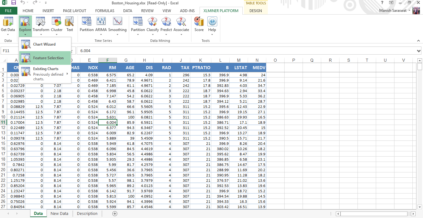
I’ve installed XLMiner. After installation, you will notice XLMINER appearing in main tabs (image below). You can also watch this overview of XLMiner platform.

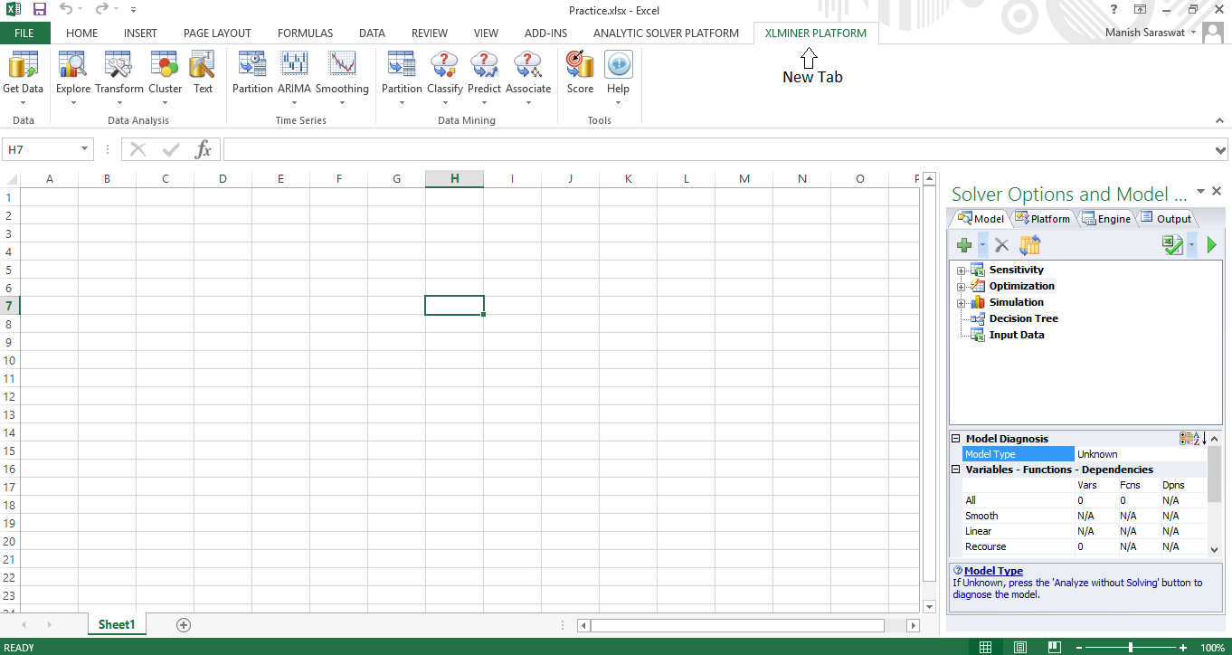
Let’s get started !

Tutorial: Multiple Linear Regression

Regression is not a big deal. You can also perform it using add-in ‘data analysis tool pack‘ available in excel. It is good for statistical analysis. For machine learning, you would need XLMiner. Here I’ve demonstrated multiple regression using XLMiner. For linear regression, all the steps remains same except you select one independent variable for modeling. Following are the steps:

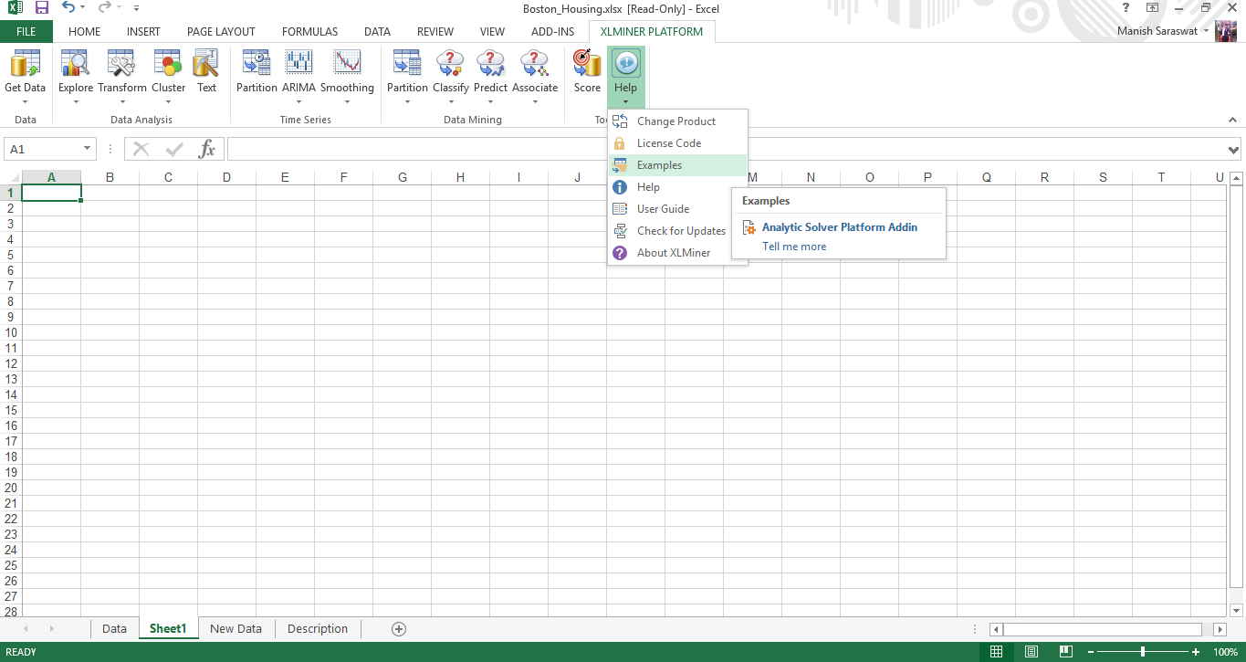
1. I’ve used Boston Housing Data Set. This data represents housing prices in Boston based on various influencing factors. You can load the data set using: Help -> Examples -> Boston Housing.

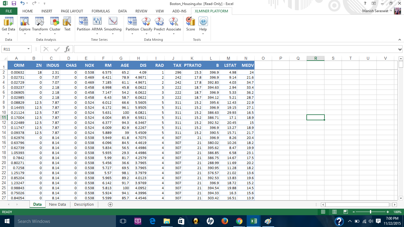
2. Here is the data set.

3. There are no missing values in this data set. However, this add-in provides a convenient option to deal with missing values. You can access this option from here.

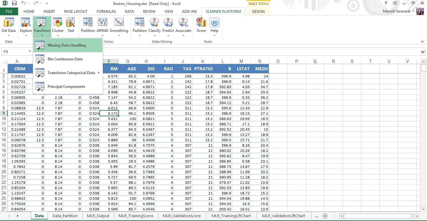
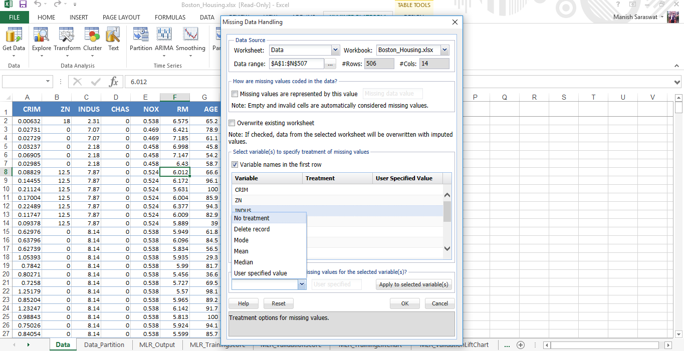
Simply, select the variables where you find missing values. If missing values are represented by ‘null’,’N/A’ or in any other form, mention it. Finally, you can choose the treatment method and done.

4. Now we’ll do feature selection. MEDV is the response variable. MEDV represents the median value of owner occupied homes in $1000.

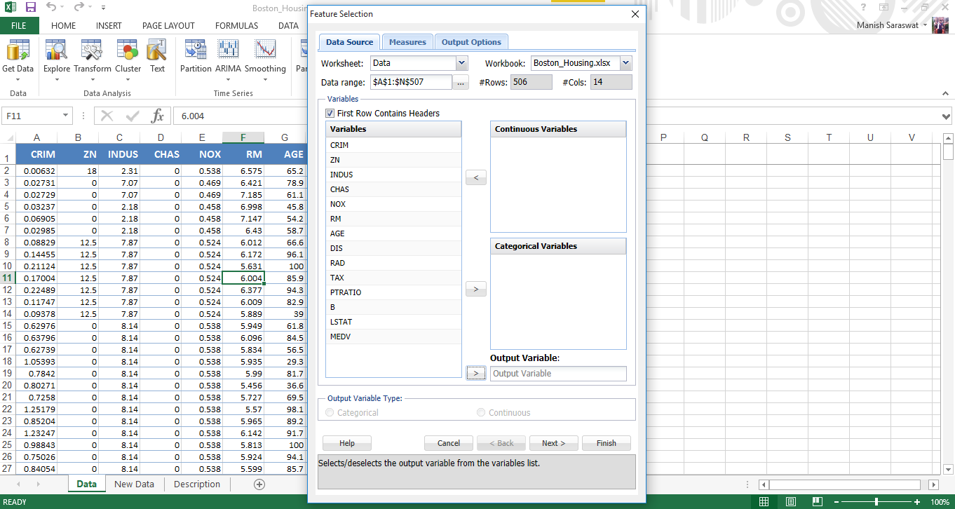
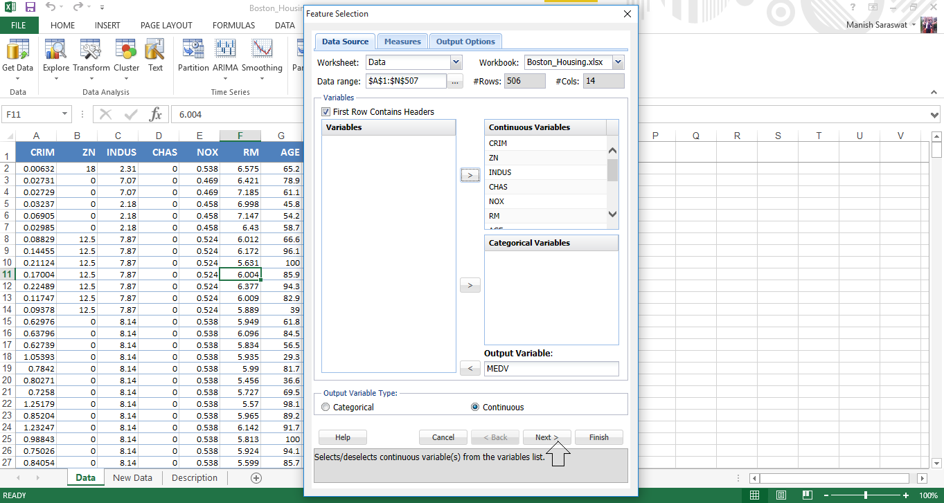
5. Use Shift + Click to select all independent variables at once. Send MEDV to Output variable. Click Next.

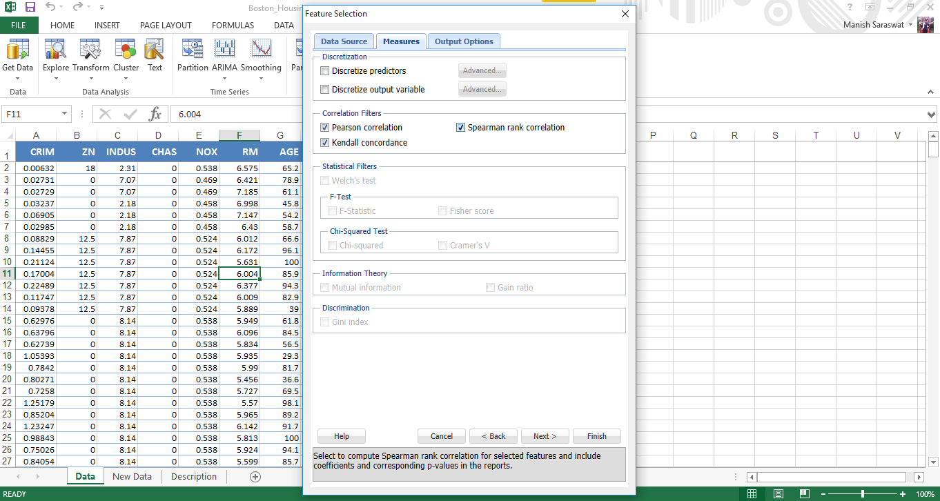
6. Select correlation filters. I’ve selected all three. Click Next

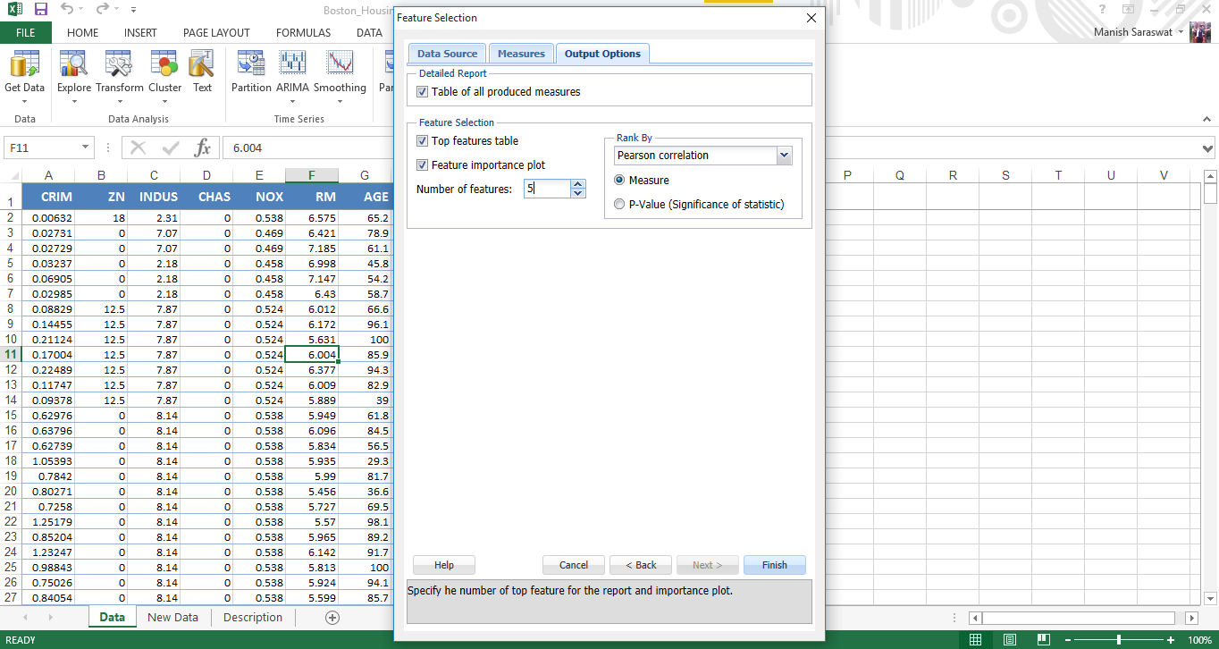
7. Now select features. Let’s find out top 5 important predictor variables. Click Finish.

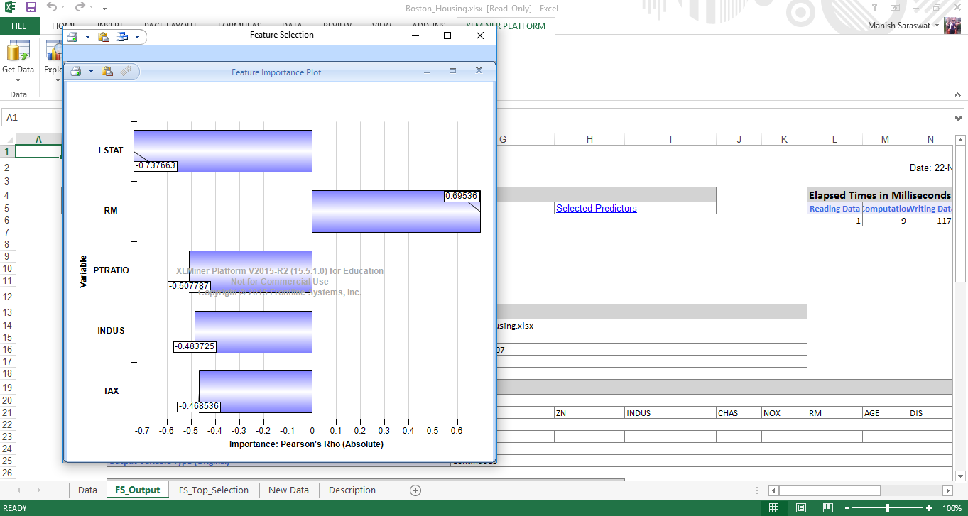
8. Here is the variable importance chart. We see, LSTAT is the most important variable, followed by RM, PTRATIO, INDUS and TAX.

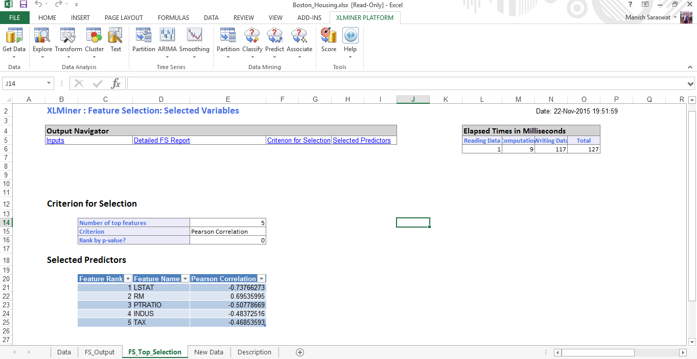
9. Close this chart. You will see Output Navigator. This helps you to navigate between various output sheets. Let’s check out ‘selected predictors’.

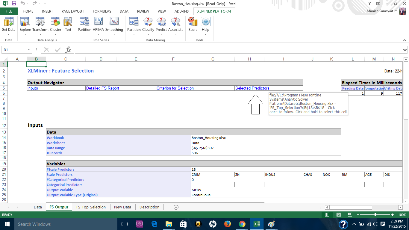
10. Here are the selected predictors. Let proceed to build a regression model using these variables.

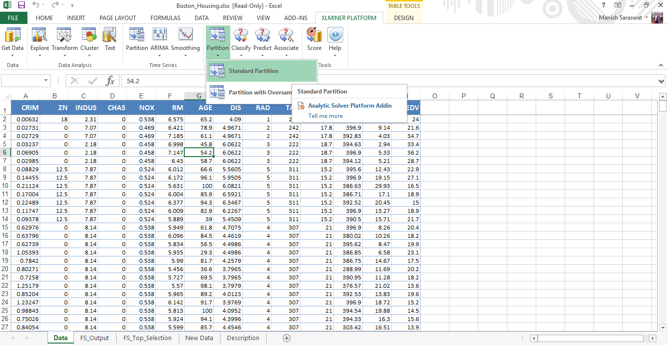
11. Prior to modeling, let’s divide (partition) this data into train and validation.

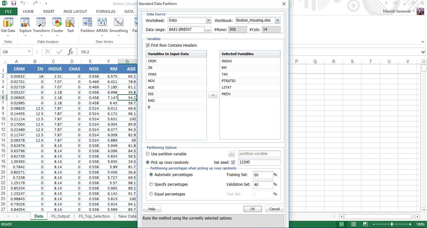
12. On the basis of feature selection, select the variables to be included in partition. Leave the rest as default values and click OK.

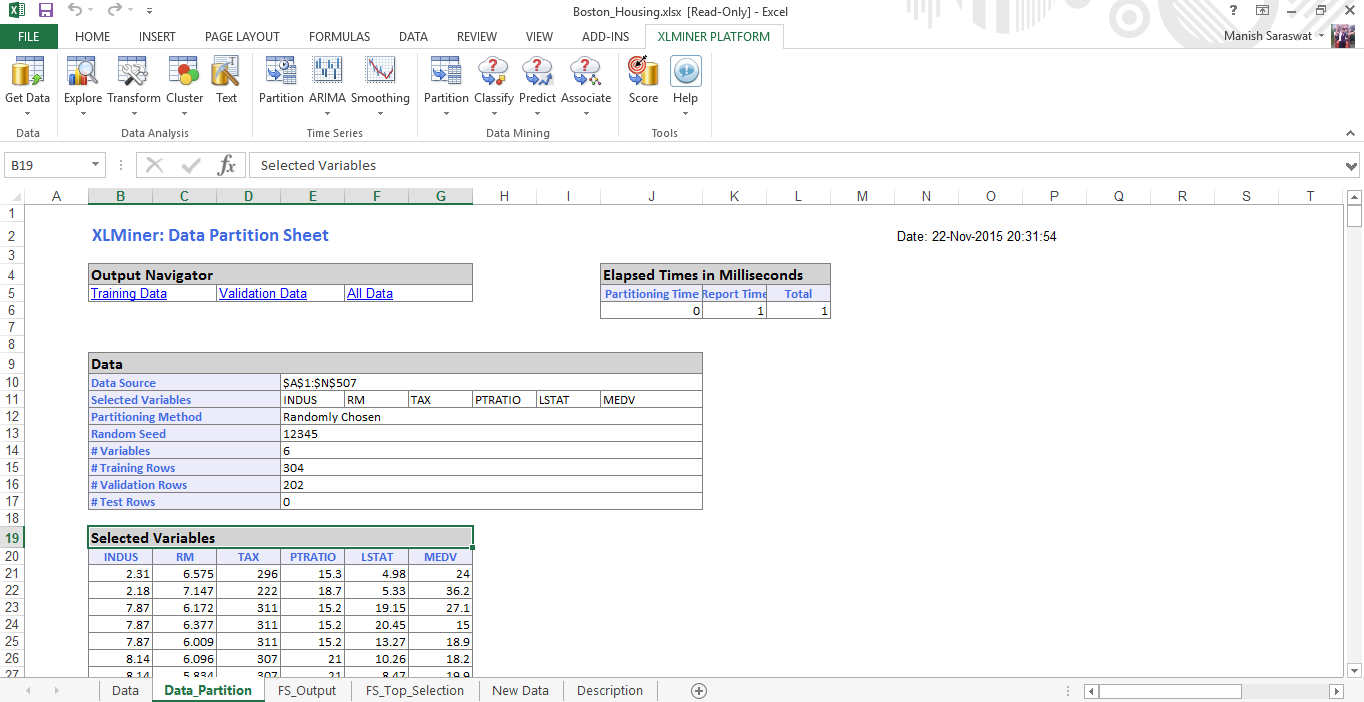
13. And, here we’ve got the training data set ready for modeling.

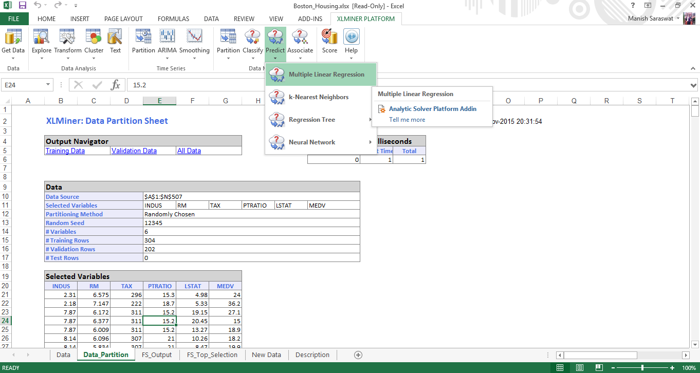
14. Click on any cell in Selected Variables and proceed to build multiple regression model. Click Multiple Linear Regression

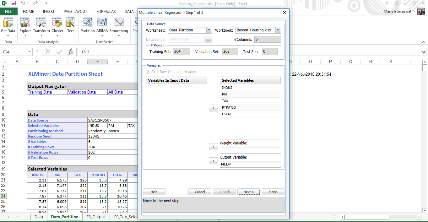
15. Select the set of predictor and response variables. Click Next

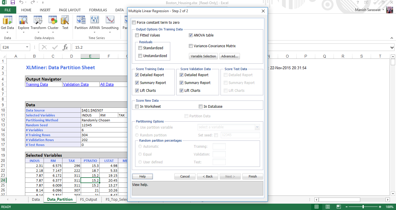
16. Select your required metrics. Click Finish

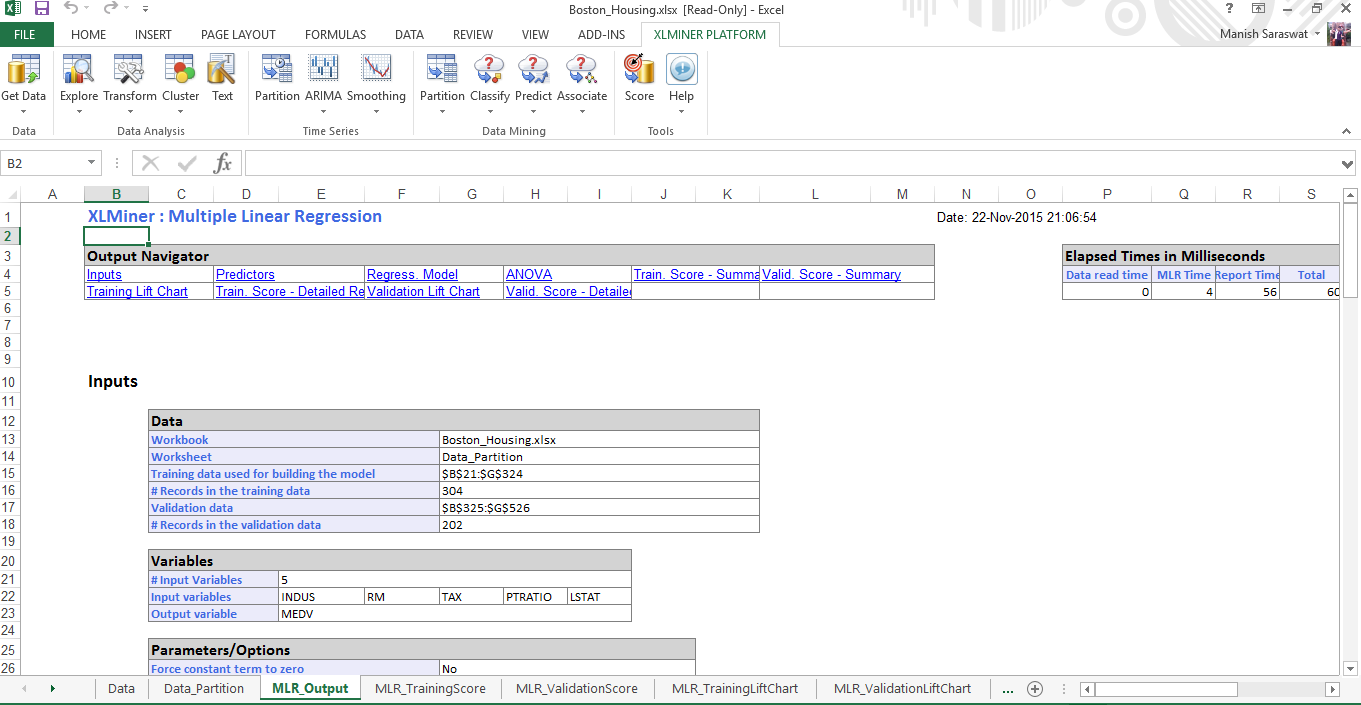
17. Your multiple linear regression model is ready. Use the output navigator to access different metrics and model accuracy.

Tutorial: Logistic Regression

Logistic Regression is a classic example of classification algorithm. Similar to multiple linear regression, below are the steps to build a logistic regression model. If you wish to quickly refresh your logistic regression concepts, you can refer to this tutorial: Simple Guide to Logistic Regression

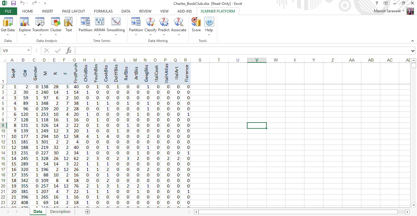
1. Load the data set ‘Charles_bookclub’. On XLMiner Ribbon, click on Help -> Example. Select this data set. This data set represents information associated with individuals who are members of a book club. We’ll build a model for predicting whether a person will purchase a book about the city of Florence based on past purchases.

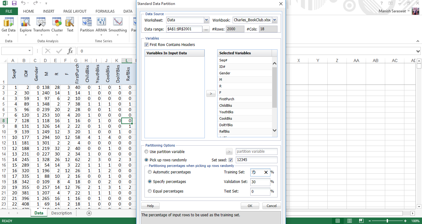
2. Now, we’ll divide the data set into training (70%) and validation (30%). This time you need to specify percentages for partition. Click OK

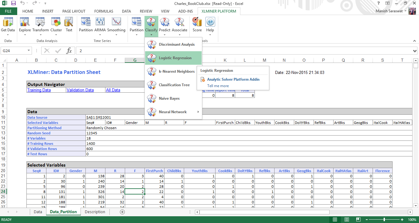
3. You’ll see a data partition sheet. Click on any cell in ‘selected variables’ table and Click on logistic regression as shown.

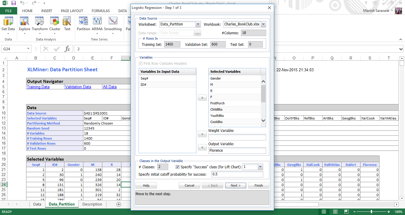
4. Here you select the input and output variables. Florence is the output variable where it gets 1 when a customer purchased a book about the city of Florence and 0 otherwise. Here 1 is success. 0 is failure as denoted in the option below. Leave the rest as default values. Click Next

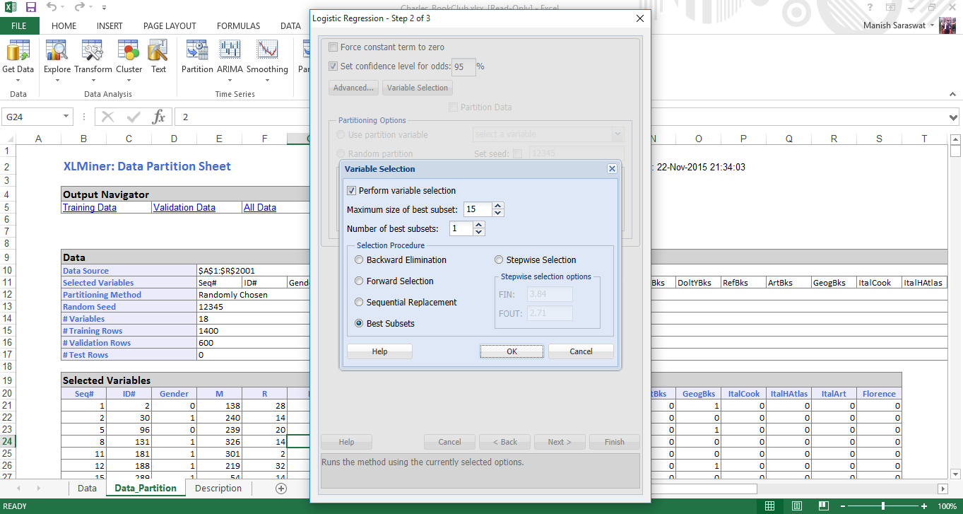
5. Select the confidence interval as 95%. If you tick ‘Force constant term to zero’, you’ll omit the constant term in the regression. Hence, don’t select it. Click on advanced, and tick ‘perform collinearity diagnostics’. It will display useful information in dealing with correlated variables having large standard errors. Click OK. Now, click Variable Selection.

6. Variable Selection helps us to deal with large number of predictor variables and find the best among them. ‘Maximum size of best subset’ takes value from 1 to N, where N is the number of input variables. We’ll not change this value. In selection procedure, you can choose any as per your preferences. I’ve chosen ‘Best Subsets’ as it searches for all combination of variables and select only the best fit ones. Click OK. Click Next.

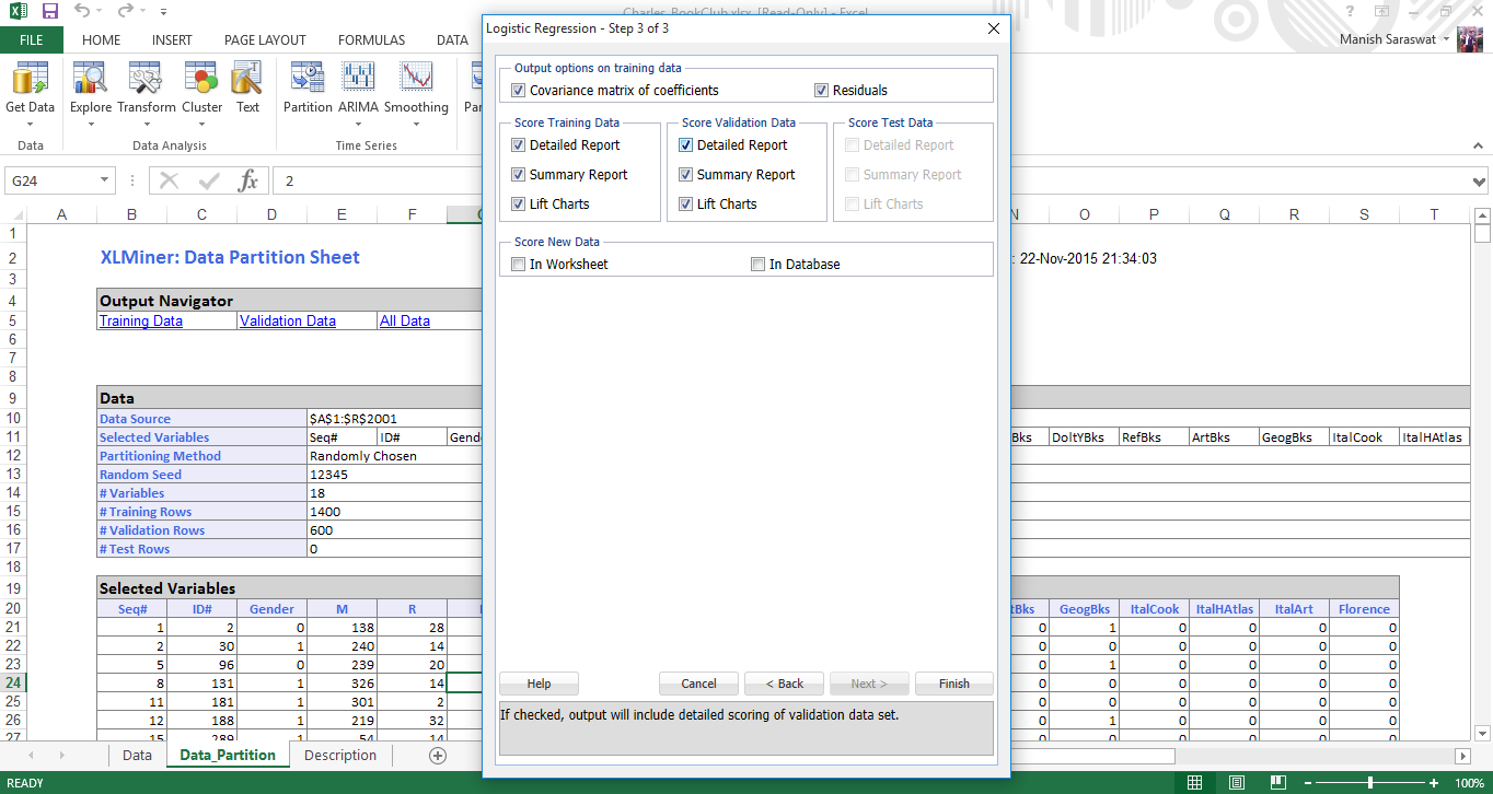
7. Now we’ll select the required computation coefficients to evaluate the model. Select Covariance matrix of coefficients and Residuals. Residuals will produce a table of fitted values and their residuals in the output. Click Finish.

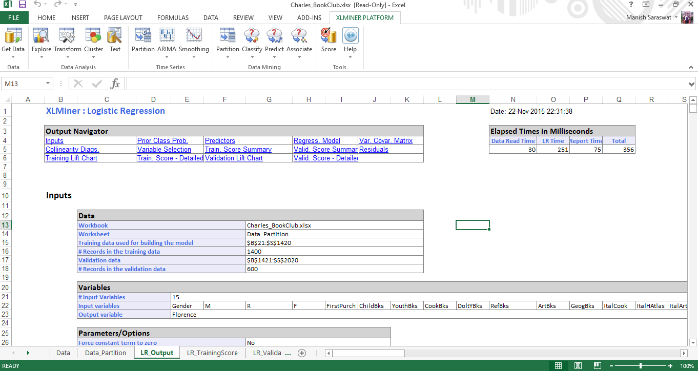
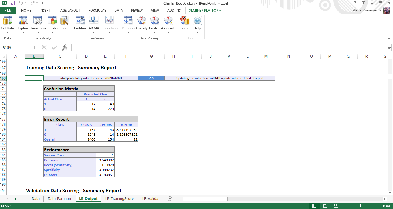
8. Here is your logistic regression model. If you scroll down this sheet, you’ll find various metrics useful to evaluate this model performance. A commonly used metric to check model’s accuracy is confusion matrix. As you scroll down, you’d find this.

Tutorial: k – Means Clustering

If you are new to clustering, here is your quick refresher to Clustering Analysis. In simple words, clustering is a technique of grouping variables with similar attributes. This technique is generally used for customer profiling and creating products as per their need.

Let’s look at the steps for perform k-means clustering in XLMiner.

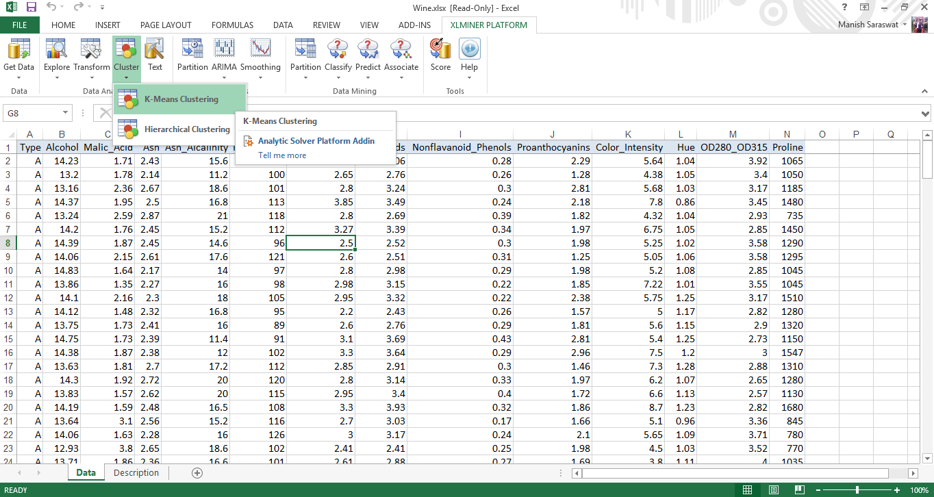
1. Load the data set Wine. Go to XLMiner ribbon, click Help -> Examples. Select Wine. In this data set, each row represents sample of wine belonging to 3 classes (A, B and C). On the basis of this data, we’ll build a clustering model to determine the class of wine. Here is the data set.

2. Click on any cell in data set. Then, click on k-means clustering.

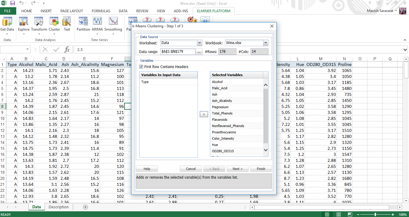
3. Type is the output variable. Hence, we’ll select all variables except Type to be used in clustering. Click Next.

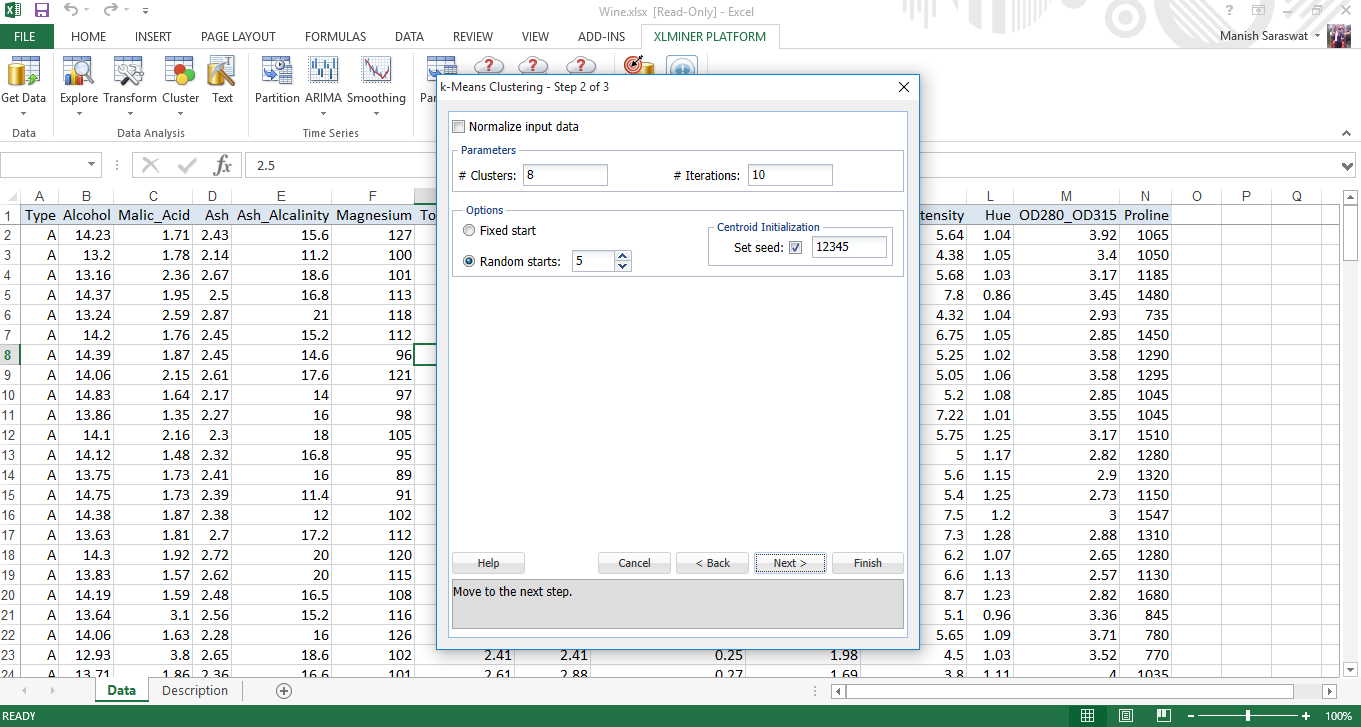
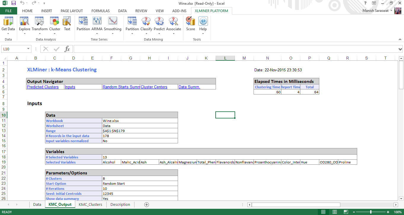
4. Let’s take number of clusters as 8. Because, with large number of clusters, sum of squared error(SSE) remains small. SSE is defined as the sum of the squared distance between each member of the cluster and its centroid. You can set any value of k, and evaluate the output from each to check which one is best. Setting random value to say 5, will let this algorithm to build the model from any random point. With this, XLMiner will generate 5 cluster sets and generate the output from best cluster. Leave the default values for rest and click Next.

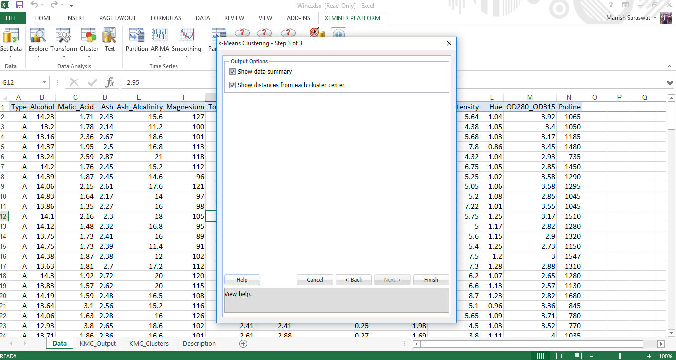
5. Leave the values as default. Click Finish

6. Here is your clustering model. Check our various evaluation metrics to determine the accuracy of this model.

Random Starts Summary: This table determines the best start with lowest sum of squares distance. In this case (#1) is the best start. Once the best start is determined, the remaining output of the model is generated using the best start as starting point.

Cluster Centers: Here you will find two boxes. The lower box shows the distance between the centroid of clusters. Larger the distance, different will be nature of clusters. For example, the difference between cluster 4 and cluster 8 is 1176.59. This suggests these clusters are very different. The upper box shows the variable values at the cluster centers.

Data Summary: It represents the average distance of observations from the center of a cluster. We can infer then cluster 2 has lowest average distance from its centroid and cluster 6 has highest.

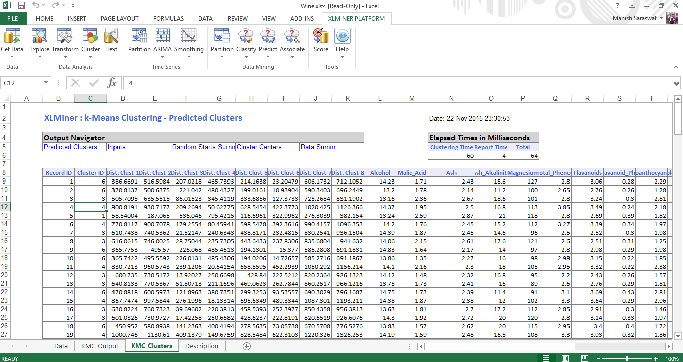
7. Click on sheet KMC_Clusters. Here you’ll find the predicted clusters. Check the Record ID 1. It has been classified to cluster 6. Because, the distance of this observation is minimum to cluster 6. Similarly, all other observations have been classified on the basis of their nearest cluster.

End Notes

I wrote this tutorial just to get your started with machine learning in excel. Once you understand these algorithms, you can easily use them in R, Python or any other programming language. Since, many of us have worked on excel at some point, it wouldn’t be difficult to understand these concepts in excel. If you get stuck, you can refer to help option in XLMiner Ribbon. The documentation is helpful and easy to understand.

Now you know the steps, I’d suggest you spend time in interpreting the model and iterate it to get the best fit. Excel might slow down with large data sets, hence you should work on small data sets as to save your time in learning.

Did you find this article useful? Have you ever worked on XLMiner? I’d love to hear your experiences and suggestions in the comments section below.

If you like what you just read & want to continue your analytics learning, subscribe to our emails, follow us on twitter or like our facebook page.