A Complete Tutorial on Time Series Modeling in R
23 minutes
Introduction
‘Time’ is the most important factor which ensures success in a business. It’s difficult to keep up with the pace of time. But, technology has developed some powerful methods using which we can ‘see things’ ahead of time. Don’t worry, I am not talking about Time Machine. Let’s be realistic here!
I’m talking about the methods of prediction & forecasting. One such method, which deals with time based data is Time Series Modeling. As the name suggests, it involves working on time (years, days, hours, minutes) based data, to derive hidden insights to make informed decision making.
Time series models are very useful models when you have serially correlated data. Most of business houses work on time series data to analyze sales number for the next year, website traffic, competition position and much more. However, it is also one of the areas, which many analysts do not understand.
So, if you aren’t sure about complete process of time series modeling, this guide would introduce you to various levels of time series modeling and its related techniques.

Table of Contents
What Is Time Series Modeling?
Let’s begin from basics. This includes stationary series, random walks , Rho Coefficient, Dickey Fuller Test of Stationarity. If these terms are already scaring you, don’t worry – they will become clear in a bit and I bet you will start enjoying the subject as I explain it.
Stationary Series
There are three basic criterion for a series to be classified as stationary series:
1. The mean of the series should not be a function of time rather should be a constant. The image below has the left hand graph satisfying the condition whereas the graph in red has a time dependent mean.

2. The variance of the series should not a be a function of time. This property is known as homoscedasticity. Following graph depicts what is and what is not a stationary series. (Notice the varying spread of distribution in the right hand graph)
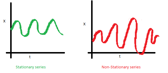
3. The covariance of the i th term and the (i + m) th term should not be a function of time. In the following graph, you will notice the spread becomes closer as the time increases. Hence, the covariance is not constant with time for the ‘red series’.

Why do I care about ‘stationarity’ of a time series?
The reason I took up this section first was that until unless your time series is stationary, you cannot build a time series model. In cases where the stationary criterion are violated, the first requisite becomes to stationarize the time series and then try stochastic models to predict this time series. There are multiple ways of bringing this stationarity. Some of them are Detrending, Differencing etc.
Random Walk
This is the most basic concept of the time series. You might know the concept well. But, I found many people in the industry who interprets random walk as a stationary process. In this section with the help of some mathematics, I will make this concept crystal clear for ever. Let’s take an example.
Example: Imagine a girl moving randomly on a giant chess board. In this case, next position of the girl is only dependent on the last position.
(Source: http://scifun.chem.wisc.edu/WOP/RandomWalk.html )
Now imagine, you are sitting in another room and are not able to see the girl. You want to predict the position of the girl with time. How accurate will you be? Of course you will become more and more inaccurate as the position of the girl changes. At t=0 you exactly know where the girl is. Next time, she can only move to 8 squares and hence your probability dips to 1/8 instead of 1 and it keeps on going down. Now let’s try to formulate this series :
X(t) = X(t-1) + Er(t)
where Er(t) is the error at time point t. This is the randomness the girl brings at every point in time.
Now, if we recursively fit in all the Xs, we will finally end up to the following equation :
X(t) = X(0) + Sum(Er(1),Er(2),Er(3).....Er(t))
Now, lets try validating our assumptions of stationary series on this random walk formulation:
1. Is the Mean constant?
E[X(t)] = E[X(0)] + Sum(E[Er(1)],E[Er(2)],E[Er(3)].....E[Er(t)])
We know that Expectation of any Error will be zero as it is random.
Hence we get E[X(t)] = E[X(0)] = Constant.
2. Is the Variance constant?
Var[X(t)] = Var[X(0)] + Sum(Var[Er(1)],Var[Er(2)],Var[Er(3)].....Var[Er(t)])
Var[X(t)] = t * Var(Error) = Time dependent.
Hence, we infer that the random walk is not a stationary process as it has a time variant variance. Also, if we check the covariance, we see that too is dependent on time.
Let’s spice up things a bit,
We already know that a random walk is a non-stationary process. Let us introduce a new coefficient in the equation to see if we can make the formulation stationary.
Introduced coefficient: Rho
X(t) = Rho * X(t-1) + Er(t)
Now, we will vary the value of Rho to see if we can make the series stationary. Here we will interpret the scatter visually and not do any test to check stationarity.
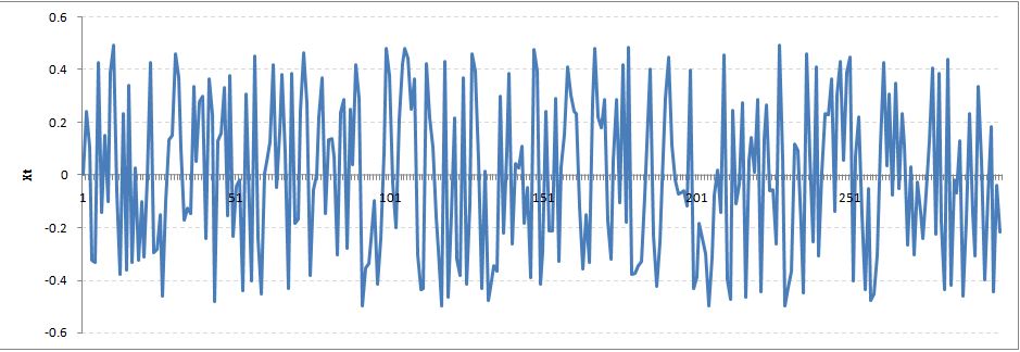
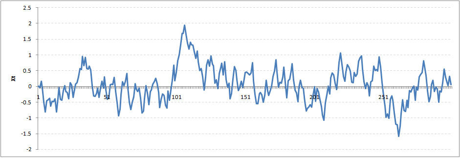
Let’s start with a perfectly stationary series with Rho = 0 . Here is the plot for the time series :
Increase the value of Rho to 0.5 gives us following graph:
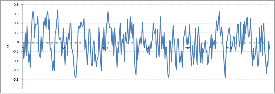
You might notice that our cycles have become broader but essentially there does not seem to be a serious violation of stationary assumptions. Let’s now take a more extreme case of Rho = 0.9
We still see that the X returns back from extreme values to zero after some intervals. This series also is not violating non-stationarity significantly. Now, let’s take a look at the random walk with rho = 1.
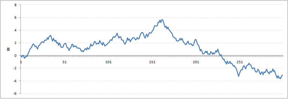
This obviously is an violation to stationary conditions. What makes rho = 1 a special case which comes out badly in stationary test? We will find the mathematical reason to this.
Let’s take expectation on each side of the equation “X(t) = Rho * X(t-1) + Er(t)”
E[X(t)] = Rho *E[ X(t-1)]
This equation is very insightful. The next X (or at time point t) is being pulled down to Rho * Last value of X.
For instance, if X(t – 1 ) = 1, E[X(t)] = 0.5 ( for Rho = 0.5) . Now, if X moves to any direction from zero, it is pulled back to zero in next step. The only component which can drive it even further is the error term. Error term is equally probable to go in either direction. What happens when the Rho becomes 1? No force can pull the X down in the next step.
Dickey Fuller Test of Stationarity
What you just learnt in the last section is formally known as Dickey Fuller test. Here is a small tweak which is made for our equation to convert it to a Dickey Fuller test:
X(t) = Rho * X(t-1) + Er(t)
=> X(t) - X(t-1) = (Rho - 1) X(t - 1) + Er(t)
We have to test if Rho – 1 is significantly different than zero or not. If the null hypothesis gets rejected, we’ll get a stationary time series.
Stationary testing and converting a series into a stationary series are the most critical processes in a time series modelling. You need to memorize each and every detail of this concept to move on to the next step of time series modelling.
Let’s now consider an example to show you what a time series looks like.
Exploration of Time Series Data in R
Here we’ll learn to handle time series data on R. Our scope will be restricted to data exploring in a time series type of data set and not go to building time series models.
I have used an inbuilt data set of R called AirPassengers. The dataset consists of monthly totals of international airline passengers, 1949 to 1960.
Loading the Data Set
Following is the code which will help you load the data set and spill out a few top level metrics.
> data(AirPassengers)
 > class(AirPassengers)
 [1] "ts"
#This tells you that the data series is in a time series format
 > start(AirPassengers)
 [1] 1949 1
#This is the start of the time series
> end(AirPassengers)
 [1] 1960 12
#This is the end of the time series
> frequency(AirPassengers)
 [1] 12
#The cycle of this time series is 12months in a year
 > summary(AirPassengers)
 Min. 1st Qu. Median Mean 3rd Qu. Max.
 104.0 180.0 265.5 280.3 360.5 622.0
Detailed Metrics
#The number of passengers are distributed across the spectrum
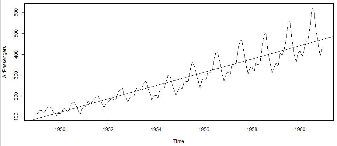
> plot(AirPassengers)
#This will plot the time series
>abline(reg=lm(AirPassengers~time(AirPassengers)))
# This will fit in a line
Here are a few more operations you can do:
> cycle(AirPassengers)
#This will print the cycle across years.
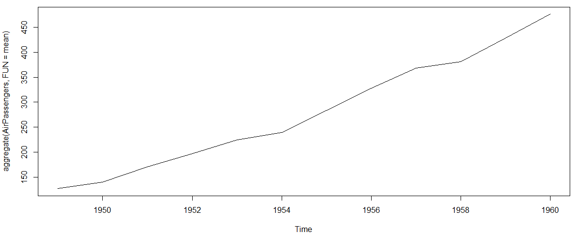
>plot(aggregate(AirPassengers,FUN=mean))
#This will aggregate the cycles and display a year on year trend
> boxplot(AirPassengers~cycle(AirPassengers))
#Box plot across months will give us a sense on seasonal effect
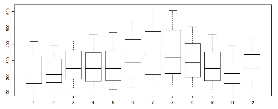
Important Inferences
- The year on year trend clearly shows that the #passengers have been increasing without fail.
- The variance and the mean value in July and August is much higher than rest of the months.
- Even though the mean value of each month is quite different their variance is small. Hence, we have strong seasonal effect with a cycle of 12 months or less.
Exploring data becomes most important in a time series model – without this exploration, you will not know whether a series is stationary or not. As in this case we already know many details about the kind of model we are looking out for.
Let’s now take up a few time series models and their characteristics. We will also take this problem forward and make a few predictions.
Introduction to ARMA Time Series Modeling
ARMA models are commonly used in time series modeling. In ARMA model, AR stands for auto-regression and MA stands for moving average. If these words sound intimidating to you, worry not – I’ll simplify these concepts in next few minutes for you!
We will now develop a knack for these terms and understand the characteristics associated with these models. But before we start, you should remember, AR or MA are not applicable on non-stationary series.
In case you get a non stationary series, you first need to stationarize the series (by taking difference / transformation) and then choose from the available time series models.
First, I’ll explain each of these two models (AR & MA) individually. Next, we will look at the characteristics of these models.
Auto-Regressive Time Series Model
Let’s understanding AR models using the case below:
The current GDP of a country say x(t) is dependent on the last year’s GDP i.e. x(t – 1). The hypothesis being that the total cost of production of products & services in a country in a fiscal year (known as GDP) is dependent on the set up of manufacturing plants / services in the previous year and the newly set up industries / plants / services in the current year. But the primary component of the GDP is the former one.
Hence, we can formally write the equation of GDP as:
x(t) = alpha * x(t – 1) + error (t)
This equation is known as AR(1) formulation. The numeral one (1) denotes that the next instance is solely dependent on the previous instance. The alpha is a coefficient which we seek so as to minimize the error function. Notice that x(t- 1) is indeed linked to x(t-2) in the same fashion. Hence, any shock to x(t) will gradually fade off in future.
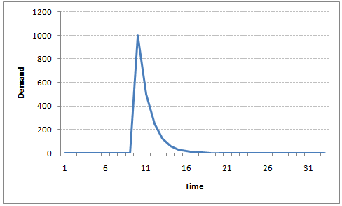
For instance, let’s say x(t) is the number of juice bottles sold in a city on a particular day. During winters, very few vendors purchased juice bottles. Suddenly, on a particular day, the temperature rose and the demand of juice bottles soared to 1000. However, after a few days, the climate became cold again. But, knowing that the people got used to drinking juice during the hot days, there were 50% of the people still drinking juice during the cold days. In following days, the proportion went down to 25% (50% of 50%) and then gradually to a small number after significant number of days. The following graph explains the inertia property of AR series:
Moving Average Time Series Model
Let’s take another case to understand Moving average time series model.
A manufacturer produces a certain type of bag, which was readily available in the market. Being a competitive market, the sale of the bag stood at zero for many days. So, one day he did some experiment with the design and produced a different type of bag. This type of bag was not available anywhere in the market. Thus, he was able to sell the entire stock of 1000 bags (lets call this as x(t) ). The demand got so high that the bag ran out of stock. As a result, some 100 odd customers couldn’t purchase this bag. Lets call this gap as the error at that time point. With time, the bag had lost its woo factor. But still few customers were left who went empty handed the previous day. Following is a simple formulation to depict the scenario :
x(t) = beta * error(t-1) + error (t)
If we try plotting this graph, it will look something like this:
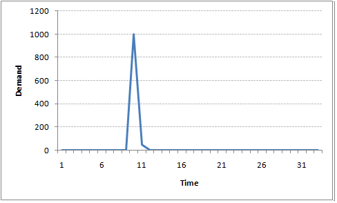
Did you notice the difference between MA and AR model? In MA model, noise / shock quickly vanishes with time. The AR model has a much lasting effect of the shock.
Difference Between AR and MA Models
The primary difference between an AR and MA model is based on the correlation between time series objects at different time points. The correlation between x(t) and x(t-n) for n > order of MA is always zero. This directly flows from the fact that covariance between x(t) and x(t-n) is zero for MA models (something which we refer from the example taken in the previous section). However, the correlation of x(t) and x(t-n) gradually declines with n becoming larger in the AR model. This difference gets exploited irrespective of having the AR model or MA model. The correlation plot can give us the order of MA model.
Exploiting ACF and PACF Plots
Once we have got the stationary time series, we must answer two primary questions:
Q1. Is it an AR or MA process?
Q2. What order of AR or MA process do we need to use?
The trick to solve these questions is available in the previous section. Didn’t you notice?
The first question can be answered using Total Correlation Chart (also known as Auto – correlation Function / ACF). ACF is a plot of total correlation between different lag functions. For instance, in GDP problem, the GDP at time point t is x(t). We are interested in the correlation of x(t) with x(t-1) , x(t-2) and so on. Now let’s reflect on what we have learnt above.
In a moving average series of lag n, we will not get any correlation between x(t) and x(t – n -1) . Hence, the total correlation chart cuts off at nth lag. So it becomes simple to find the lag for a MA series. For an AR series this correlation will gradually go down without any cut off value. So what do we do if it is an AR series?
Here is the second trick. If we find out the partial correlation of each lag, it will cut off after the degree of AR series. For instance,if we have a AR(1) series, if we exclude the effect of 1st lag (x (t-1) ), our 2nd lag (x (t-2) ) is independent of x(t). Hence, the partial correlation function (PACF) will drop sharply after the 1st lag. Following are the examples which will clarify any doubts you have on this concept :
ACF PACF
The blue line above shows significantly different values than zero. Clearly, the graph above has a cut off on PACF curve after 2nd lag which means this is mostly an AR(2) process.
ACF PACF
Clearly, the graph above has a cut off on ACF curve after 2nd lag which means this is mostly a MA(2) process.
Till now, we have covered on how to identify the type of stationary series using ACF & PACF plots. Now, I’ll introduce you to a comprehensive framework to build a time series model. In addition, we’ll also discuss about the practical applications of time series modelling.
Framework and Application of ARIMA Time Series Modeling
A quick revision, Till here we’ve learnt basics of time series modeling, time series in R and ARMA modeling. Now is the time to join these pieces and make an interesting story.
Overview of the Framework
This framework(shown below) specifies the step by step approach on ‘How to do a Time Series Analysis‘:
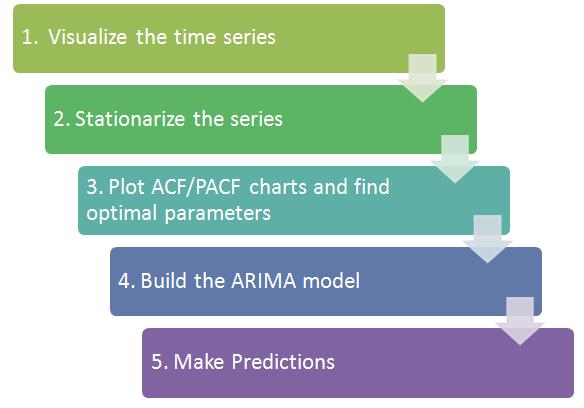
As you would be aware, the first three steps have already been discussed above. Nevertheless, the same has been delineated briefly below:
Step 1: Visualize the Time Series
It is essential to analyze the trends prior to building any kind of time series model. The details we are interested in pertains to any kind of trend, seasonality or random behaviour in the series. We have covered this part in the second part of this series.
Step 2: Stationarize the Series
Once we know the patterns, trends, cycles and seasonality , we can check if the series is stationary or not. Dickey – Fuller is one of the popular test to check the same. We have covered this test in the first part of this article series. This doesn’t ends here! What if the series is found to be non-stationary?
There are three commonly used technique to make a time series stationary:
1. Detrending : Here, we simply remove the trend component from the time series. For instance, the equation of my time series is:
x(t) = (mean + trend * t) + error
We’ll simply remove the part in the parentheses and build model for the rest.
2. Differencing : This is the commonly used technique to remove non-stationarity. Here we try to model the differences of the terms and not the actual term. For instance,
x(t) – x(t-1) = ARMA (p , q)
This differencing is called as the Integration part in AR(I)MA. Now, we have three parameters
p : AR
d : I
q : MA
3. Seasonality: Seasonality can easily be incorporated in the ARIMA model directly. More on this has been discussed in the applications part below.
Step 3: Find Optimal Parameters
The parameters p,d,q can be found using ACF and PACF plots. An addition to this approach is can be, if both ACF and PACF decreases gradually, it indicates that we need to make the time series stationary and introduce a value to “d”.
Step 4: Build ARIMA Model
With the parameters in hand, we can now try to build ARIMA model. The value found in the previous section might be an approximate estimate and we need to explore more (p,d,q) combinations. The one with the lowest BIC and AIC should be our choice. We can also try some models with a seasonal component. Just in case, we notice any seasonality in ACF/PACF plots.
Step 5: Make Predictions
Once we have the final ARIMA model, we are now ready to make predictions on the future time points. We can also visualize the trends to cross validate if the model works fine.
Applications of Time Series Model
Now, we’ll use the same example that we have used above. Then, using time series, we’ll make future predictions. We recommend you to check out the example before proceeding further.
Where did we start?
Following is the plot of the number of passengers with years. Try and make observations on this plot before moving further in the article.
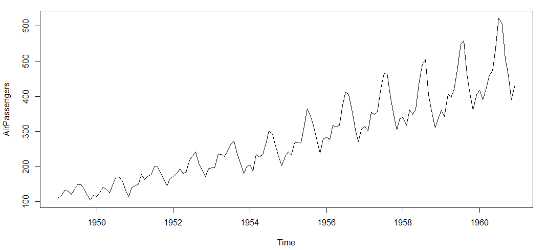
Here are my observations:
1. There is a trend component which grows the passenger year by year.
2. There looks to be a seasonal component which has a cycle less than 12 months.
3. The variance in the data keeps on increasing with time.
We know that we need to address two issues before we test stationary series. One, we need to remove unequal variances. We do this using log of the series. Two, we need to address the trend component. We do this by taking difference of the series. Now, let’s test the resultant series.
adf.test(diff(log(AirPassengers)), alternative="stationary", k=0)
Augmented Dickey-Fuller Test
data: diff(log(AirPassengers))
 Dickey-Fuller = -9.6003, Lag order = 0,
 p-value = 0.01
 alternative hypothesis: stationary
We see that the series is stationary enough to do any kind of time series modelling.
Next step is to find the right parameters to be used in the ARIMA model. We already know that the ‘d’ component is 1 as we need 1 difference to make the series stationary. We do this using the Correlation plots. Following are the ACF plots for the series:
#ACF Plots
acf(log(AirPassengers))
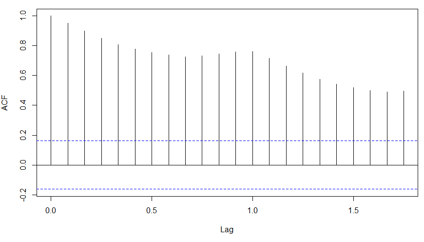
What do you see in the chart shown above?
Clearly, the decay of ACF chart is very slow, which means that the population is not stationary. We have already discussed above that we now intend to regress on the difference of logs rather than log directly. Let’s see how ACF and PACF curve come out after regressing on the difference.
acf(diff(log(AirPassengers)))
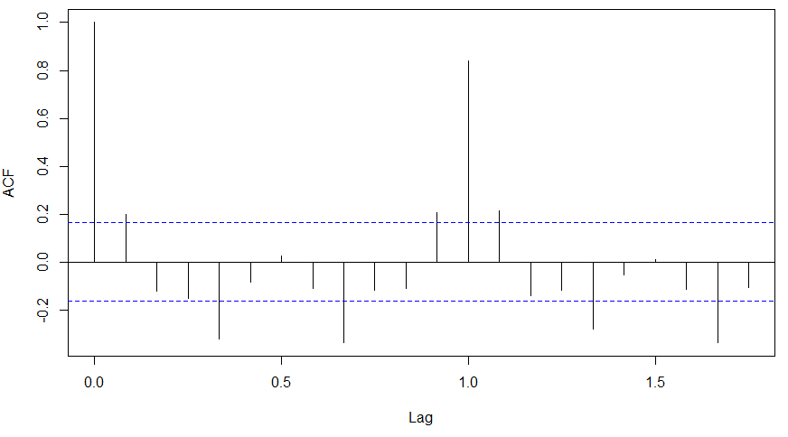
pacf(diff(log(AirPassengers)))
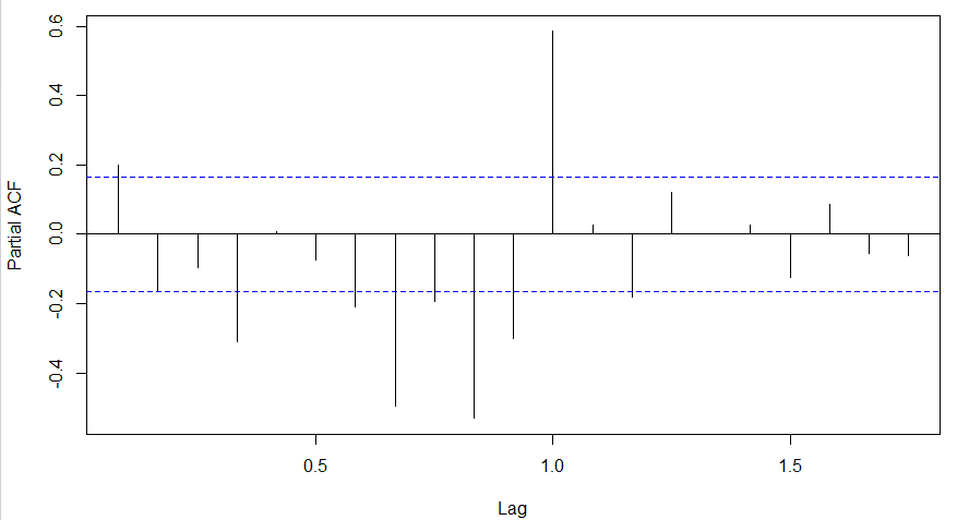
Clearly, ACF plot cuts off after the first lag. Hence, we understood that value of p should be 0 as the ACF is the curve getting a cut off. While value of q should be 1 or 2. After a few iterations, we found that (0,1,1) as (p,d,q) comes out to be the combination with least AIC and BIC.
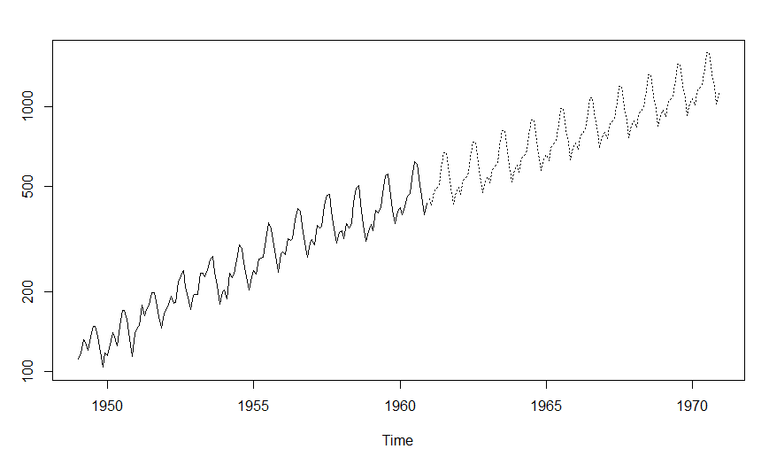
Let’s fit an ARIMA model and predict the future 10 years. Also, we will try fitting in a seasonal component in the ARIMA formulation. Then, we will visualize the prediction along with the training data. You can use the following code to do the same :
(fit <- arima(log(AirPassengers), c(0, 1, 1),seasonal = list(order = c(0, 1, 1), period = 12)))
pred <- predict(fit, n.ahead = 10*12)
ts.plot(AirPassengers,2.718^pred$pred, log = "y", lty = c(1,3))
Practice Projects
Now, its time to take the plunge and actually play with some other real datasets. So are you ready to take on the challenge? Test the techniques discussed in this post and accelerate your learning in Time Series Analysis with the following Practice Problems:
 | Practice Problem: Food Demand Forecasting Challenge | Forecast the demand of meals for a meal delivery company |
 | Practice Problem: Time Series Analyses | Forecast the passenger traffic for an intra-city rail system |
Conclusion
With this, we come to this end of tutorial on Time Series Modelling. I hope this will help you to improve your knowledge to work on time based data. To reap maximum benefits out of this tutorial, I’d suggest you to practice these R codes side by side and check your progress.
Frequently Asked Questions
A. Time series modeling refers to building a machine learning model that can auto-generate future predictions based on existing or historical data.
A. ARIMA stands for Auto-Regressive Integrated Moving Average. It is a model that does time series forecasting by converting a non-stationary time series into a stationary one.
A. Here are the basic steps to do a Time Series Analysis:
Step 1: Visualize the time series
Step 2: Stationarize the series
Step 3: Find optimal parameters
Step 4: Build ARIMA model
Step 5: Make predictions
Tavish Srivastava, co-founder and Chief Strategy Officer of Analytics Vidhya, is an IIT Madras graduate and a passionate data-science professional with 8+ years of diverse experience in markets including the US, India and Singapore, domains including Digital Acquisitions, Customer Servicing and Customer Management, and industry including Retail Banking, Credit Cards and Insurance. He is fascinated by the idea of artificial intelligence inspired by human intelligence and enjoys every discussion, theory or even movie related to this idea.


Really useful. Please also write on how to make weather data into a times series for further analysis in R
This blog does not explain how to create a time series 'object', using a ts() function. Eg: exchange <- ts(exchange_data, frequency=_, start=c(Start_date, begining_value)). exchange_data is the data, frequency is the number of observations per year, start date is the start year and begining_value is the starting nuber of the unit of observation (eg first month for monthly observations)
I would like to read a similar article.
Hi I am a medical specialist (MD Pediatrics) with further training in research and statistics (Panjab University, Chandigarh). In our medical settings, time series data are often seen in ICU and anesthesia related research where patients are continuously monitored for days or even weeks generating such data. Frankly speaking, your article has clearly decoded this arcane process of time series analysis with quite wonderful insight into its practical relevance. Fabulous article Mr Tavish, kindly write more about ARIMA modelling. Thanks a lot Dr Sahul Bharti
great article to start with timeseries mod
Awesome Tutorial. Big fan of you Tavish, your articles are really great. Explanations in beautiful manner.
Please elucidate on PACF part of MA series. Thanks
PACF is not really required for MA models, as the degree of MA can be found from ACF directly.
Hi Tavish. First off all, congratulations on your work around here. It's been very useful. Thank you I a doubt and i hope that you can help me I performed a Dickey-Fuller test on both series ; AirPassengers and diff( log(AirPassengers)) Here the results: Augmented Dickey-Fuller Test data: diff(log(AirPassengers)) Dickey-Fuller = -9.6003, Lag order = 0, p-value = 0.01 alternative hypothesis: stationary and Augmented Dickey-Fuller Test data: diff(log(AirPassengers)) Dickey-Fuller = -9.6003, Lag order = 0, p-value = 0.01 alternative hypothesis: stationary In both tests i got a small p-value that allows me to reject the non stationary hypothesis. Am I right? If so, the first series is already stationary?? This means that if i had performed a stationary test on the original series had move on to the next step. Thank you in advance.
Now with the right results . Augmented Dickey-Fuller Test data: AirPassengers Dickey-Fuller = -4.6392, Lag order = 0, p-value = 0.01 alternative hypothesis: stationary Augmented Dickey-Fuller Test data: diff(log(AirPassengers)) Dickey-Fuller = -9.6003, Lag order = 0, p-value = 0.01 alternative hypothesis: stationary
Fortunately the auto.arima function allows us to model time series quite nicely though it is quite useful to know the basics. Here is some code I wrote on the same data http://rpubs.com/ajaydecis/ts
Awesome Tavish! Short, crisp and absolutely crystal clear :)
Thanks for the post. Awesome explanation..!
Rohit, Please be more specific, and provide the location of the discussion on lnkd, so that Tavish can respond appropriately.. .
The pairs of graphs introducing the concepts worked really well. I found the use of english letters for all the formulae clear.
Hi, thanks for the tutorial. I have just one comment for the identification of MA order. We have been taught that the length of the first line of the ACF curve is always equal to 1 [because it's cov(Xt, Xt)/(sigma(Xt)*sigma(Xt) = 1]. So we dont look at this line, we start counting after this line. If that's the case, your first MA example should be MA(1) instead of MA(2)
Hi Tavish, One question about the ADF test. adf.test(diff(log(AirPassengers)), alternative="stationary", k=0) How shall we decide on the value for k? I tried to run another version with no specification of k value. And the default value used it k = 5 (aka. lag order = 5). Many thanks!
Thank you. Your article is great
Is there any way we can get a PDF of this? I would like to use it to introduce my staff to trend analysis and some errors to look out for--
Why did we take d as 1 in this example?
We have difference the series once and get to see that the trend is removed. Had the trend been still there we would have difference the series once again. This series did not require to be difference more than once; hence d=1.
This article was very helpful
why the author not answer the questions..... this force us to look for better articles and doubt this one.
Please explain the parameters to this last line of code ts.plot(AirPassengers,2.718^pred$pred, log = "y", lty = c(1,3))
Hi, After you run this pred <- predict(APmodel, n.ahead=10*12) take a look at 'pred' It is a list of 2 (pred and se - I assume these are predictions and errors.) I would suggest using a name other than pred in the predict function to avoid confusion , I used the following APforecast <- predict(APmodel, n.ahead=10*12) So APforecast is a list of pred and se and we need to plot the pred values , ie APforecast$pred Also we did the arima on log of AirPassengers, so the forecast we have got is actually log of the true forecast. Hence we need to find the log inverse of what we have got. ie. log(forecast) = APforecast$pred so forecast = e ^ APforecast$pred e= 2.718 If you find that confusing, I would suggest reading up on natural logarithms and their inverse the log = "y' is to plot on a logarithmic scale - this is not needed, try the function without it and with and observe the results. The lty bit I have not figured out yet. Drop it and try the ts.plot, it works fine.
Hey Amy, ts.plot() will plot several time series on the same plot. The first two entries are the two time series he's plotting. The last two entries are nice visual parameters (we'll come back to that). Clearly, this plots the AirPassengers time series in a dark, continuous line. The second entry is also a time series, but it is a little more confusing: " 2.718^pred$pred". First, you have to know what pred$pred is. The function predict() here is a generic function that will work differently for different classes plugged into it (it says so if you type ?predict). The class we're working with is an Arima class. If you type ?predict.Arima you will find a good description of what the function is all about. predict.Arima() spits out something with a "pred" part (for predict) and a "se" part (for standard error). We want the "pred" part, hence pred$pred. So, pred$pred is a time series. Now, 2.718^pred$pred is also. You have to remember that 2.718 is approximately the constant e, and then this makes sense. He's just undoing the log that he placed on the data when he created "fit". As for the last two parameters, log = "y" sets the y-axis to be on a log scale. And finally, lty = c(1,3) will set the LineTYpe to 1 (for solid) for the original time series and 3 (for dotted) for the predicted time series.
Thanks a lot! Very useful article.
Hi, It is very interesting. Can you make the same example with Python code?
Hi Tavish, Thank you very much for the nice explanation about time series using ARIMA. However I have the following the queries regarding the analysis. 1.ACF and PACF are to find the p and q values as part of ARIMA? Is only ACF is not enough to find the p and q? If not can you explain the importance of PACF? Thanks in advance.......:)
if non stationarity is present in data ,can we analyse that data
Hey Tavish, really enjoyed the content, Just a small doubt: Can you please ebaorate the covariance in stationary terms. I understand the covariance term, but here in time series,it is not coming to my mind. Can you please help me understand the third condition of stationary series i.e "The covariance of the i th term and the (i + m) th term should not be a function of time." Please help me understand from data perspective e.g if i have sales data for each date. how can you explain convariance in real life example with daily sales data.
Hi Tavish,Thanks a lot .This article was immensely helpful . I just had one small issue.After the last step, If I want to extract the predicted values from the curve . How do we do that?
@Parth, You get the predicted values from the variable pred. pred is a list with two items: pred and se. ( prediction and standard error). To see the predictions, use this command: print(pred$pred)
Hi Ram, Thanks for your help . Yeah, print(pred$pred) would give us log of the predicted values. print(2.718^pred$pred) would give us the actual predicted values. Thanks
how to extract the data for the predicted and actual values from R
hello, the data you used in your tutorial, AirPassengers, is already a time series object. my question is, HOW can i make/prepare my own time series object? i currently have a historical currency exchange data set, with first column being date, and the rest 20 columns are titled by country, and their values are the exchange rate. after i convert my date column into date object, when i use the same commands used in your tutorial, the results are funny. for example, start(data$Date) will give me a result of: [1] 1 1 and frequency(data$Date) will return: [1] 1 can you please explain HOW to prepare our data accordingly so we can use the functions? thank you!
If you type in ?ts then you should be on your way. You only need a (single) time series, a frequency, and a start date. The examples at the bottom of the documentation should be very helpful. I'm guessing you'd write something like ts( your_timeseries_data, frequency = 365, start = c(1980, 153)) for instance if your data started on the 153rd day of 1980.
Thank you very much...
What is the format of your date value before you converted it ? If you post a few rows from your data, perhaps we can help.
Thank you, It was very helpful for me :-)
Hi, thanks for the article! I'm still unclear how the parameters (p,d,q) = (0,1,1) were found from the ACF and PCF. I understand d, but not p or q. What do you mean when you say 'cutting off'?
Hi Kevin, ACF plot is a bar chart of the coefficients of correlation between a time series and lags of itself. PACF plot is a plot of the partial correlation coefficients between the series and lags of itself. To find p and q you need to look at ACF and PACF plots. The interpretation of ACF and PACF plots to find p and q are as follows: AR (p) model: If ACF plot tails off* but PACF plot cut off** after p lags MA(q) model: If PACF plot tails off but ACF plot cut off after q lags ARMA(p,q) model: If both ACF and PACF plot tail off, you can choose different combinations of p and q , smaller p and q are tried. ARIMA(p,d,q) model: If it's ARMA with d times differencing to make time series stationary. Use AIC and BIC to find the most appropriate model. Lower values of AIC and BIC are desirable. *Tails of mean slow decaying of the plot, i.e. plot has significant spikes at higher lags too. **Cut off means the bar is significant at lag p and not significant at any higher order lags. Here is a link that might help you understand the concept further http://people.duke.edu/~rnau/arimrule.htm Hope this helps.
Hi. Great article and I am working on a gforce (values + and -) dataset and am having trouble with the log function. NaNs produced and not sure how to go about addressing this. Any help would be appreciated.
GREAT ARTICLE... THANK YOU TAVISH!!!! One strong suggestion to Analytics Vidya. Please add a link of PDF downloads to these kind of articles (without advertisements) which for a person like me who is creating a repository of awesome articles to learn from will be really helpful!!!!
Hi Tavish, Great article. I had one doubt .In the last step , while fitting the arima model , you have used log(AirPassengers) instead of diff(log(AirPassengers)). Why is that so? log(Airpassengers) isn't a stationary series , right?
Just an FYI for r-newbies. I don't think its mentioned above by to run adf.test you will need to install the tseries package.
Many thanks, I was just looking for that info!
It;s handled by defining c(0, 1, 1) while fitting. Here 1st 1 denote to differentiation, which will make series stationary.
Which software is best for Time Series Analysis. I am using EViews that's why unable to understand the executions from your website. Many thanks in anticipation!
Hi Tavish . This article is really helpful. I just had one doubt. In the last step, why are we applying an ARIMA model on log(AirPassengers) rather than diff(log(AirPassengers)). It's diff(log(AirPassengers)) that is stationary , right ? One more thing, how are we fitting the seasonal component? Thanks
Hi Tavish! Great Work. Can you guide us with Multivariate Time Series model as well. (I'm relatively new to this field) I have Pharma Drug sales to be forecasted . I'm unable to find relevant techniques anywhere.
Hi, I'm unable to run "adf.test(diff(log(AirPassengers)), alternative = "stationary", k=0))". please suggest.... regards rohit
Hi, My question is on ACF Plot. When I look at any ACF graph, the first plot always exceeds the blue dotted lines. I would like to know the reason for the same. Thanks Amit
This is a very useful and quite thorough guide. It helped me a lot. The author, thank you very much!
Hi All, Some times other variables also impact on forecasting besides Date, Churn. For example, We want to find out Churn , the following are variables to compute forecasting 1)Date , 2)Churn, 3)No.of Contracts_Expire. ( No. of contracts are going to expire date wise) 4) No_Customers_Getting_Price_Up, ( We have the data date wise No. of customers are getting Price up in future) 5) Competitor_Price(It is Adhoc), 6) WeekDay/WorkingDay, ( 7)Holiday/Not ....... Thank
What is good web site get the more comprehensive details on Time Series using R. Thanks Kumar
Very insightful article, I work for a retail and wholesale bank in South Africa and haven't looked at time series analysis in years. I'm currently doing some work observing the relationship between different risk types over time. This was quite a nice little refresher.
Why cant we just use auto.arima to arrive at the appropriate values for p,d,q ??
Thank for your article!! I have one question. You writed " adf.test(diff(log(AirPassengers)), alternative="stationary", k=0)" . It's mean you created model with diff(log(AirPassengers)). But below your code, you created ARIMA model "arima(log(AirPassengers), c(0, 1, 1), seasonal = list(order = c(0, 1, 1), period = 12))". Please tell why did yoy write. I want to know that Stationary series test use diff(log(AirPassengers) data , but ARIMA model use log(AirPassengers).
In the conclusion, both ACF and PACF cutoff at 1. Since ACF cutoffs at 1,we can infer that q(MA) is 1, but how can we say that p (AR) is 0 as we need to look at PACF which suggests p to be 1. But p is concluded to be 0 which is in contrast to the PACF conclusion. Plz enlighten. TIA.
Hi, Does time series depend only upon time and not on any other parameters? Like if we have to forecast Sales, should we consider other factors like Promotions, festivals, shop loacation etc while building the ARIMA model? Only time should be considered?
Really amazing. I am now more clear about these concepts. Very nice explanation.
Nice article, for the biginners. I really appreciate this great writeup.
Please, how can i get the predicted values in a normal form to conpare with the original airpassengers values?
An article with a very relevant theme and especially with excellent didactics for content transmission. Please Mr. Mr Tavish, write other articles like these on time series. It will certainly be appreciated by many professionals. Thank you. Paulo Moniz (data scientist)
hi Being a r newbie, I have a small query. I have a 100 year data set of temperature. I want to remove the auto corelation of data. Can i use ar1 for it???Please advice and steps to be done for removing the autocorelation
Hi Tavish, It's a great article. I've a little question, why do you use log(AirPassengers) instead of diff(log(AirPassengers)) to build the model? (fit <- arima(log(AirPassengers), c(0, 1, 1),seasonal = list(order = c(0, 1, 1), period = 12))) Thank you! Eva
ts.plot(AirPassengers,2.718^pred$pred, log = "y", lty = c(1,3)) Can someone please clarify what is the use of the following in the above function: 1. 2.718 (Where did this number come from? & why is it needed?) 2. log = "y" (Again, meaning & use?) 3. lty = c(1, 3) (same question) Finally, when I used the Ljung-Box test, the p-value was 2.2x e^(-16); which is very small thus signifying a high degree of autocorrelation in the residuals. From what I've read, it is highly undesirable. Any further references & reading material which explains how to deal with it? Thanks in advance
GREAT ARTICLE AND TEACHING CAPACITY. I ENJOYED IT
Hi I am a Research Scholar. Please any one help me to provide ARIMA model and Feed Forwad Neural Network Code in r programming. my email id is [email protected]