Kaggle Solution: What’s Cooking ? (Text Mining Competition)

Introduction

Tutorial on Text Mining, XGBoost and Ensemble Modeling in R

I came across What’s Cooking competition on Kaggle last week. At first, I was intrigued by its name. I checked it and realized that this competition is about to finish. My bad! It was a text mining competition.  This competition went live for 103 days and ended on 20th December 2015.

Still, I decided to test my skills. I downloaded the data set, built a model and managed to get a score of 0.79817 in the end. Even though, my submission wasn’t accepted after the competition got over, but I could check my score. This got me in top 20 percentile.

I used Text Mining, XGBoost and Ensemble Modeling to get this score. And, I used R. It took me less than 6 hours to achieve this milestone. I teamed up with Rohit Hinduja, who is currently interning at Analytics Vidhya.

To help beginners in R, here is my solution in a tutorial format. In the article below, I’ve adapted a step by step methodology to explain the solution. This tutorial requires prior knowledge of R and Machine Learning.

I am confident that this tutorial can improve your R coding skills and approaches.

Let’s get started.

Before you start…

Here’s a quick approach to (for beginners) give a tough fight in any kaggle competition:

1. Get comfortable with Statistics
2. Learn and Understand the 7 steps of Data Exploration
3. Become proficient with any one of the language Python, R or SAS (or the tool of your choice).
4. Learn to use basic ML Algorithms
5. Learn Text Mining.
6. Identify the right competition first according to your skills. Here’s a good read: Kaggle Competitions: How and where to begin?

What’s Cooking ?

Yeah! I could smell, it was a text mining competition. The data set had a list of id, ingredients and cuisine. There were 20 types of cuisine in the data set. The participants were asked to predict a cuisine based on available ingredients.

The ingredients were available in the form of a text list. That’s where text mining was used. Before reaching to the modeling stage, I cleaned the text using pre-processing methods. And, finally with available set of variables, I used an ensemble of XGBoost Models.

Note: My system configuration is core i5 processor, 8GB RAM and 1TB Hard Disk. 

Solution

Below is the my solution of this competition:

Step 1. Hypothesis Generation

Though many people don’t believe in this, but this step do wonders when done intuitively. Hypothesis Generation can help you to think ‘out of data’. It also helps you understand the data and relationship between the variables. It should ideally be done after you’ve looked at problem statement (but not the data).

Before exploring data, you must think smartly on the problem statement. What could be the features which can influence your outcome variable? Think on these terms and write down your findings. I did the same. Below is my list of findings which I thought could help me in determining a cuisine:

1. Taste: Different cuisines are cooked to taste different. If you know the taste of the food, you can estimate the type of cuisine.
2. Smell: With smell also, we can determine a cuisine type
3. Serving Type: We can identify the cuisine by looking at the way it is being served. What are the dips it is served with?
4. Hot or Cold: Some cuisines are served hot while some cold.
5. Group of ingredients and spices: Precisely, after one has tasted, we can figure out the cuisine by the mix of ingredients used. For example, you are unlikely to find pasta as an ingredient in any Indian cooking.
6. Liquid Served: Some cuisines are represented by the type of drinks served with food.
7. Location: The location of eating can be a factor in determining cuisine.
8. Duration of cooking: Some cuisines tend to have longer cooking cycles. Others might have more fast food style cooking.
9. Order of pouring ingredients: At times, the same set of ingredients are poured in a different order in different cuisines.
10. Percentage of ingredients which are staple crops / animals in the country of the cuisine:  A lot of cooking historically has been developed based on the availability of the ingredients in the country. A high percentage here could be a good indicator.

Step 2. Download and Understand the Data Set

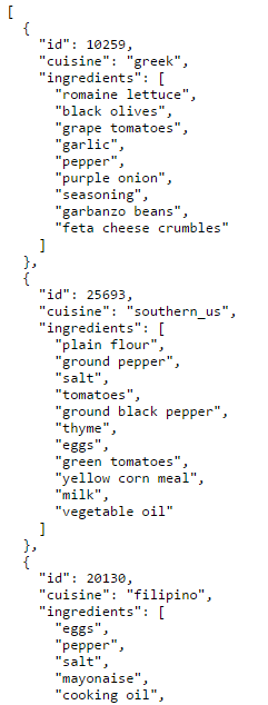
The data set shows a list of id, cuisine and ingredients . The data set is available in json format. The dependent variable is cuisine. The independent variable is ingredients. Train data set is used for creating model. Test data is used to checking the accuracy of the model. If you are still confused between the two, remember, test data set do not have dependent variable.

Since the data is available in text format, I was determined to quickly build a corpus of ingredients (next step). Here is a snapshot of data set for your perusal in json format:

Step 3. Basics of Text Mining

For this solution, I’ve used R (precisely R Studio 0.99.484) in Windows environment.

Text Mining / Natural Language Processing helps computers to understand text and derive useful information from it. Several brands use this technique to analyse customer sentiments on social media. It consists of pre-defined set of commands used to clean the data. Since, text mining is mainly used to verify sentiments, the incoming data can be loosely structured, multilingual, textual or might have poor spellings.

Some of the commonly used techniques in text mining are:

1. Bag of Words : This techniques creates a ‘bag’ or group of words by counting the number of times each word has appear and use these counts as independent variables.
2. Change the text case : Data is often received in irregular formats. For example: ‘CyCLe’ & ‘cycle’. Both means the same thing but is represented in an irregular manner. Hence, it is advisable to change the case of text. Either to upper or lower case.
3. Deal with Punctuation : This can be tricky at times. Your tool(R or Python) would read ‘data mining’ & ‘data-mining’ as two different words. But they are same. Hence, we should remove the punctuation elements also.
4. Remove Stopwords : Stopwords are nothing but the words which add no value to text. They don’t describe any sentiment. Examples are ‘i’,’me’,’myself’,’they’,’them’ and many more. Hence, we should remove such words too. In addition to stopwords, you may find other words which are repeated  but add no value. Remove them as well.
5. Stemming or Lemmatization : This suggests bringing a word back to its root. It is generally used of words which are similar but only differ by tenses. For example: ‘play’, ‘playing’ and ‘played’ can be stemmed into one word ‘play’, since all three connotes the same action.

I’ve used these techniques in my solution too.

Step 4. Importing and Combining Data Set

Since the data set is in json format, I require different set of libraries to perform this step. jsonlite offers an easy way to import data in R. This is how I’ve done:

1. Import Train and Test Data Set

setwd('D:/Kaggle/Cooking')

install.packages('jsonlite')
library(jsonlite)

train <- fromJSON("train.json")
test <- fromJSON("test.json")

2. Combine both train and test data set. This will make our text cleaning process less painful. If I do not combine, I’ll have to clean train and test data set separately. And, this would take a lot of time.

But I need to add the dependent variable in test data set. Data can be combine using rbind (row-bind) function.

#add dependent variable
test$cuisine <- NA
#combine data set
combi <- rbind(train, test)

Step 5. Pre-Processing using tm package ( Text Mining)

As explained above, here are the steps used to clean the list of ingredients. I’ve used tm package for text mining.

1. Create a Corpus of Ingredients (Text)

#install package
library(tm)
#create corpus
corpus <- Corpus(VectorSource(combi$ingredients))

2.  Convert text to lowercase

corpus <- tm_map(corpus, tolower)
corpus[[1]]

3. Remove Punctuation

corpus <- tm_map(corpus, removePunctuation)
corpus[[1]]

4.  Remove Stopwords

corpus <- tm_map(corpus, removeWords, c(stopwords('english')))
corpus[[1]]

5. Remove Whitespaces

corpus <- tm_map(corpus, stripWhitespace)
corpus[[1]]

6. Perform Stemming

corpus <- tm_map(corpus, stemDocument)
corpus[[1]]

6. After we are done with pre-processing, it is necessary to convert the text into plain text document. This helps in pre-processing documents as text documents.

corpus <- tm_map(corpus, PlainTextDocument)

7. For further processing, we’ll create a document matrix where the text will categorized in columns

#document matrix
frequencies <- DocumentTermMatrix(corpus) 
frequencies

Step 6. Data Exploration

1. Computing frequency column wise to get the ingredient with highest frequency

#organizing frequency of terms
freq <- colSums(as.matrix(frequencies))
length(freq)

ord <- order(freq)
ord

#if you wish to export the matrix (to see how it looks) to an excel file
m <- as.matrix(frequencies)
dim(m) write.csv(m, file = 'matrix.csv')

#check most and least frequent words
freq[head(ord)]
freq[tail(ord)]

#check our table of 20 frequencies
head(table(freq),20)
tail(table(freq),20)

We see that, there are may terms (ingredients) which occurs once, twice or thrice. Such ingredients won’t add any value to the model. However, we need to be sure about removing these ingredients as it might cause loss in data. Hence, I’ll remove only the terms having frequency less than 3

#remove sparse terms
sparse <- removeSparseTerms(frequencies, 1 - 3/nrow(frequencies))
dim(sparse)

2. Let’s visualize the data now. But first, we’ll create a data frame.

#create a data frame for visualization
wf <- data.frame(word = names(freq), freq = freq)
head(wf)

#plot terms which appear atleast 10,000 times
library(ggplot2)

chart <- ggplot(subset(wf, freq >10000), aes(x = word, y = freq))
chart <- chart + geom_bar(stat = 'identity', color = 'black', fill = 'white')
chart <- chart + theme(axis.text.x=element_text(angle=45, hjust=1))
chart

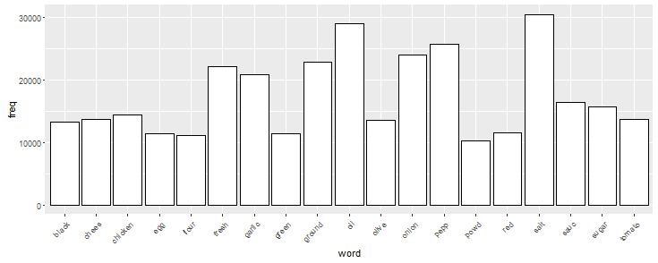
Here we see that salt, oil, pepper are among the highest occurring ingredients. You can change the freq values (in graph above) to visualize the frequency of ingredients.

3. We can also find the level of correlation between two ingredients. For example, if you have any ingredient in mind which can be highly correlated with others, we can find it. Here I am checking the correlation of salt and oil with other variables. I’ve assigned the correlation limit as 0.30. It means, I’ll only get the value which have correlation higher than 0.30.

#find associated terms
findAssocs(frequencies, c('salt','oil'), corlimit=0.30)

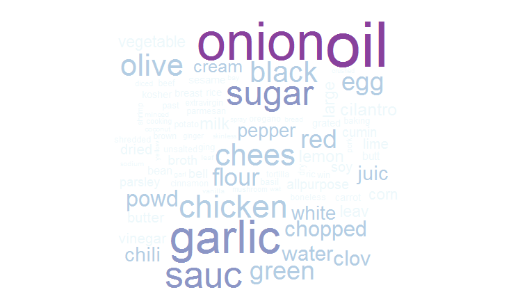
4. We can also create a word cloud to check the most frequent terms. It is easy to build and gives an enhanced understanding of ingredients in this data. For this, I’ve used the package ‘wordcloud’.

#create wordcloud
library(wordcloud)
set.seed(142)

#plot word cloud
wordcloud(names(freq), freq, min.freq = 2500, scale = c(6, .1), colors = brewer.pal(4, "BuPu"))

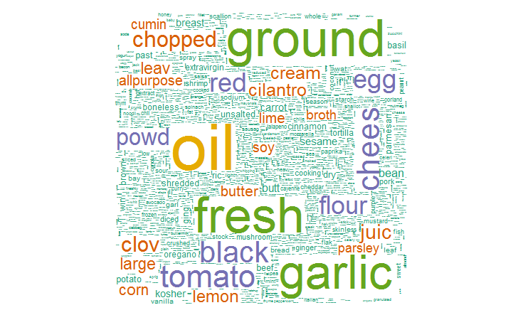
#plot 5000 most used words
wordcloud(names(freq), freq, max.words = 5000, scale = c(6, .1), colors = brewer.pal(6, 'Dark2'))

5. Now I’ll make final structural changes in the data.

#create sparse as data frame
newsparse <- as.data.frame(as.matrix(sparse))
dim(newsparse)

#check if all words are appropriate
colnames(newsparse) <- make.names(colnames(newsparse))

#check for the dominant dependent variable
table(train$cuisine)

Here I find that, ‘italian’ is the most popular in all the cuisine available. Using this information, I’ve added the dependent variable ‘cuisine’ in the data frame newsparse as ‘italian’.

#add cuisine
newsparse$cuisine <- as.factor(c(train$cuisine, rep('italian', nrow(test))))

#split data 
mytrain <- newsparse[1:nrow(train),]
mytest <- newsparse[-(1:nrow(train)),]

Step 7. Model Building

As my first attempt, I couldn’t think of any algorithm better than naive bayes. Since I have a multi class categorical variable, I expected naive bayes to do wonders. But, to my surprise, the naive bayes model went in perpetuity. Perhaps, my machine specifications aren’t powerful enough.

Next, I tried Boosting. Thankfully, the model computed without any trouble. Boosting is a technique which convert weak learners into strong learners. In simple terms, I built three XGBoost model. All there were weak, means their accuracy weren’t good. I combined (ensemble) the predictions of three model to produce a strong model.  To know more about boosting, you can refer to this introduction.

The reason I used boosting is because, it works great on sparse matrices. Since, I’ve a sparse matrix here, I expected it to give good results. Sparse Matrix is a matrix which has large number of zeroes in it. It’s opposite is dense matrix. In a dense matrix, we have very few zeroes. XGBoost, precisely, deliver exceptional results on sparse matrices.

I did parameter tuning on XGBoost model to ensure that every model behaves in a different way. To read more on XGBoost, here’s a comprehensive documentation: XGBoost

Below is my complete code. I’ve used the packages xgboost and matrix. The package ‘matrix’ is used to create sparse matrix quickly.

library(xgboost)
library(Matrix)

Now, I’ve created a sparse matrix using xgb.DMatrix of train data set. I’ve kept the set of independent variables and removed the dependent variable.

# creating the matrix for training the model
ctrain <- xgb.DMatrix(Matrix(data.matrix(mytrain[,!colnames(mytrain) %in% c('cuisine')])), label = as.numeric(mytrain$cuisine)-1)

I’ve created a sparse matrix for test data set too. This is done to create a watchlist. Watchlist is a list of sparse form of train and test data set. It is served as an parameter in xgboost model to provide train and test error as the model runs.

#advanced data set preparation
dtest <- xgb.DMatrix(Matrix(data.matrix(mytest[,!colnames(mytest) %in% c('cuisine')]))) 
watchlist <- list(train = ctrain, test = dtest)

To understand the modeling part, I suggest you to read this document. I’ve built 3 just models with different parameters . You can even create 40 – 50 models for ensembling. In the code below, I’ve used ‘Objective = multi:softmax’. Because, this is a case of multi classification.

Among other parameters, eta, min_child_weight, max.depth and gamma directly controls the model complexity. These parameters prevents the model to overfit. The model will be more conservative, if these values are chosen larger.

#train multiclass model using softmax
#first model
xgbmodel <- xgboost(data = ctrain, max.depth = 25, eta = 0.3, nround = 200, objective = "multi:softmax", num_class = 20, verbose = 1, watchlist = watchlist)

#second model
xgbmodel2 <- xgboost(data = ctrain, max.depth = 20, eta = 0.2, nrounds = 250, objective = "multi:softmax", num_class = 20, watchlist = watchlist)

#third model
xgbmodel3 <- xgboost(data = ctrain, max.depth = 25, gamma = 2, min_child_weight = 2, eta = 0.1, nround = 250, objective = "multi:softmax", num_class = 20, verbose = 2,watchlist = watchlist)

#predict 1
xgbmodel.predict <- predict(xgbmodel, newdata = data.matrix(mytest[, !colnames(mytest) %in% c('cuisine')]))
xgbmodel.predict.text <- levels(mytrain$cuisine)[xgbmodel.predict + 1]

#predict 2
xgbmodel.predict2 <- predict(xgbmodel2, newdata = data.matrix(mytest[, !colnames(mytest) %in% c('cuisine')])) 
xgbmodel.predict2.text <- levels(mytrain$cuisine)[xgbmodel.predict2 + 1]

#predict 3
xgbmodel.predict3 <- predict(xgbmodel3, newdata = data.matrix(mytest[, !colnames(mytest) %in% c('cuisine')])) 
xgbmodel.predict3.text <- levels(mytrain$cuisine)[xgbmodel.predict3 + 1]

#data frame for predict 1
submit_match1 <- cbind(as.data.frame(test$id), as.data.frame(xgbmodel.predict.text))
colnames(submit_match1) <- c('id','cuisine')
submit_match1 <- data.table(submit_match1, key = 'id')

#data frame for predict 2
submit_match2 <- cbind(as.data.frame(test$id), as.data.frame(xgbmodel.predict2.text))
colnames(submit_match2) <- c('id','cuisine')
submit_match2 <- data.table(submit_match2, key = 'id')

#data frame for predict 3
submit_match3 <- cbind(as.data.frame(test$id), as.data.frame(xgbmodel.predict3.text))
colnames(submit_match3) <- c('id','cuisine')
submit_match3 <- data.table(submit_match3, key = 'id')

Now I have three weak learners. You can check their accuracy using:

sum(diag(table(mytest$cuisine, xgbmodel.predict)))/nrow(mytest) 
sum(diag(table(mytest$cuisine, xgbmodel.predict2)))/nrow(mytest)
sum(diag(table(mytest$cuisine, xgbmodel.predict3)))/nrow(mytest)

The simple key is ensemble. Now, I have three data frame for model predict, predict2 and predict 3. I’ve now extracted the ‘cuisine’ column from predict and predict 2 into predict 3. With this step, I get all values of ‘cuisines’ in one data frame. Now I can easily ensemble their predictions

#ensembling 
submit_match3$cuisine2 <- submit_match2$cuisine 
submit_match3$cuisine1 <- submit_match1$cuisine

I’ve used the MODE function to extract the predicted value with highest frequency per id.

#function to find the maximum value row wise
Mode <- function(x) {
u <- unique(x)
u[which.max(tabulate(match(x, u)))]
}

x <- Mode(submit_match3[,c("cuisine","cuisine2","cuisine1")])

y <- apply(submit_match3,1,Mode)

final_submit <- data.frame(id= submit_match3$id, cuisine = y)
#view submission file
data.table(final_submit)

#final submission
write.csv(final_submit, 'ensemble.csv', row.names = FALSE)

After following the step mentioned above, you can easily get the same score as mine (0.798). You would have seen, I haven’t used any brainy method to improve this model. i just applied my basics. Since I’ve just started, I would like to see if I can push this further the highest level now.

End Notes

With this, I finish this tutorial for now! There are many things in this data set which you can try at your end. Due to time constraints, I couldn’t spent much time on it during the competition. But, it’s time you put on your thinking boots. I failed at Naive Bayes. So, why don’t you create an ensemble of naive bayes models? or may be, create a cluster of ingredients and build a model over it ?

I’m sure this strategy might give you a better score. Perhaps, more knowledge. In this tutorial, I’ve built a predictive model on What’s Cooking ? data set hosted by Kaggle. I took a step wise approach to cover various stages of model building. I used text mining and ensemble of 3 XGBoost models. XGBoost in itself is a deep topic. I plan to cover it deeply in my forthcoming articles. I’d suggest you to practice and learn.

Did you find the article useful? Share with us if you have done similar kind of analysis before. Do let us know your thoughts about this article in the box below.

If you like what you just read & want to continue your analytics learning, subscribe to our emails, follow us on twitter or like our facebook page.