Ridge and Lasso Regression in Python | Complete Tutorial (Updated 2024)
Last week, I saw a recorded talk at NYC Data Science Academy from Owen Zhang, Chief Product Officer at DataRobot. He said, ‘if you are using regression without regularization, you have to be very special!’. I hope you get what a person of his stature referred to. I understood it very well and decided to explore regularization techniques in detail. In this article, I have explained the complex science behind ‘Ridge Regression‘ and ‘Lasso Regression, ‘ which are the most fundamental regularization techniques used in data science, sadly still not used by many.
Learning Objectives
- Learn the concepts of Ridge and Lasso Regression and their role in regularizing linear regression models.
- Understand the differences between Ridge and Lasso regression, including the penalty term used in each approach and how it affects the regression model coefficients.
- Learn how to implement Ridge and Lasso Regression in Python using the scikit-learn library.
Table of contents
- What Are Ridge Regression and Lasso Regression?
- Why Penalize the Magnitude of Coefficients?
- How Does Ridge Regression Work?
- How Does Lasso Regression Work?
- Some Underlying Mathematical Principles
- Sample Project to Apply Your Regression Skills
- Comparison Between Ridge Regression and Lasso Regression
- Conclusion
- Frequently Asked Questions
What Are Ridge Regression and Lasso Regression?
When we talk about regression, we often end up discussing Linear and Logistic Regression, as they are the most popular of the 7 types of regressions. In this article, we’ll focus on Ridge and Lasso regression, which are powerful techniques generally used for creating parsimonious models in the presence of a ‘large’ number of features. Here ‘large’ can typically mean either of two things:
- Large enough to enhance the tendency of a model to overfit (as low as 10 variables might cause overfitting)
- Large enough to cause computational challenges. With modern systems, this situation might arise in the case of millions or billions of features.
Though Ridge and Lasso might appear to work towards a common goal, the inherent properties and practical use cases differ substantially. If you’ve heard of them before, you must know that they work by penalizing the magnitude of coefficients of features and minimizing the error between predicted and actual observations. These are called ‘regularization’ techniques.
Lasso regression is a regularization technique. It is used over regression methods for a more accurate prediction. This model uses shrinkage. Shrinkage is where data values are shrunk towards a central point as the mean. The lasso procedure encourages simple, sparse models (i.e. models with fewer parameters).
Regularization Techniques
The key difference is in how they assign penalties to the coefficients:
- Ridge Regression:
- Performs L2 regularization, i.e., adds penalty equivalent to the square of the magnitude of coefficients
- Minimization objective = LS Obj + α * (sum of square of coefficients)
- Lasso Regression:
- Performs L1 regularization, i.e., adds penalty equivalent to the absolute value of the magnitude of coefficients
- Minimization objective = LS Obj + α * (sum of the absolute value of coefficients)
Here, LS Obj refers to the ‘least squares objective,’ i.e., the linear regression objective without regularization.
If terms like ‘penalty’ and ‘regularization’ seem very unfamiliar to you, don’t worry; we’ll discuss these in more detail throughout this article. Before digging further into how they work, let’s try to understand why penalizing the magnitude of coefficients should work in the first place.
Why Penalize the Magnitude of Coefficients?
Let’s try to understand the impact of model complexity on the magnitude of coefficients. As an example, I have simulated a sine curve (between 60° and 300°) and added some random noise using the following code:
Python Code
This resembles a sine curve but not exactly because of the noise. We’ll use this as an example to test different scenarios in this article. Let’s try to estimate the sine function using polynomial regression with powers of x from 1 to 15. Let’s add a column for each power upto 15 in our dataframe. This can be accomplished using the following code:
Add a Column for Each Power upto 15
for i in range(2,16):  #power of 1 is already there
    colname = 'x_%d'%i      #new var will be x_power
    data[colname] = data['x']**i
print(data.head())add a column for each power upto 15
The dataframe looks like this:
Making 15 Different Linear Regression Models
Now that we have all the 15 powers, let’s make 15 different linear regression models, with each model containing variables with powers of x from 1 to the particular model number. For example, the feature set of model 8 will be – {x, x_2, x_3, …, x_8}.
First, we’ll define a generic function that takes in the required maximum power of x as an input and returns a list containing – [ model RSS, intercept, coef_x, coef_x2, … upto entered power ]. Here RSS refers to the ‘Residual Sum of Squares,’ which is nothing but the sum of squares of errors between the predicted and actual values in the training data set and is known as the cost function or the loss function. The python code defining the function is:
#Import Linear Regression model from scikit-learn.
from sklearn.linear_model import LinearRegression
def linear_regression(data, power, models_to_plot):
    #initialize predictors:
    predictors=['x']
    if power>=2:
        predictors.extend(['x_%d'%i for i in range(2,power+1)])

    #Fit the model
    linreg = LinearRegression(normalize=True)
    linreg.fit(data[predictors],data['y'])
    y_pred = linreg.predict(data[predictors])

    #Check if a plot is to be made for the entered power
    if power in models_to_plot:
        plt.subplot(models_to_plot[power])
        plt.tight_layout()
        plt.plot(data['x'],y_pred)
        plt.plot(data['x'],data['y'],'.')
        plt.title('Plot for power: %d'%power)

    #Return the result in pre-defined format
    rss = sum((y_pred-data['y'])**2)
    ret = [rss]
    ret.extend([linreg.intercept_])
    ret.extend(linreg.coef_)
    return ret
Note that this function will not plot the model fit for all the powers but will return the RSS and coefficient values for all the models. I’ll skip the details of the code for now to maintain brevity. I’ll be happy to discuss the same through the comments below if required.
Store all the Results in Pandas Dataframe
Now, we can make all 15 models and compare the results. For ease of analysis, we’ll store all the results in a Pandas dataframe and plot 6 models to get an idea of the trend. Consider the following code:
#Initialize a dataframe to store the results:
col = ['rss','intercept'] + ['coef_x_%d'%i for i in range(1,16)]
ind = ['model_pow_%d'%i for i in range(1,16)]
coef_matrix_simple = pd.DataFrame(index=ind, columns=col)

#Define the powers for which a plot is required:
models_to_plot = {1:231,3:232,6:233,9:234,12:235,15:236}

#Iterate through all powers and assimilate results
for i in range(1,16):
    coef_matrix_simple.iloc[i-1,0:i+2] = linear_regression(data, power=i, models_to_plot=models_to_plot)
We would expect the models with increasing complexity to better fit the data and result in lower RSS values. This can be verified by looking at the plots generated for 6 models:
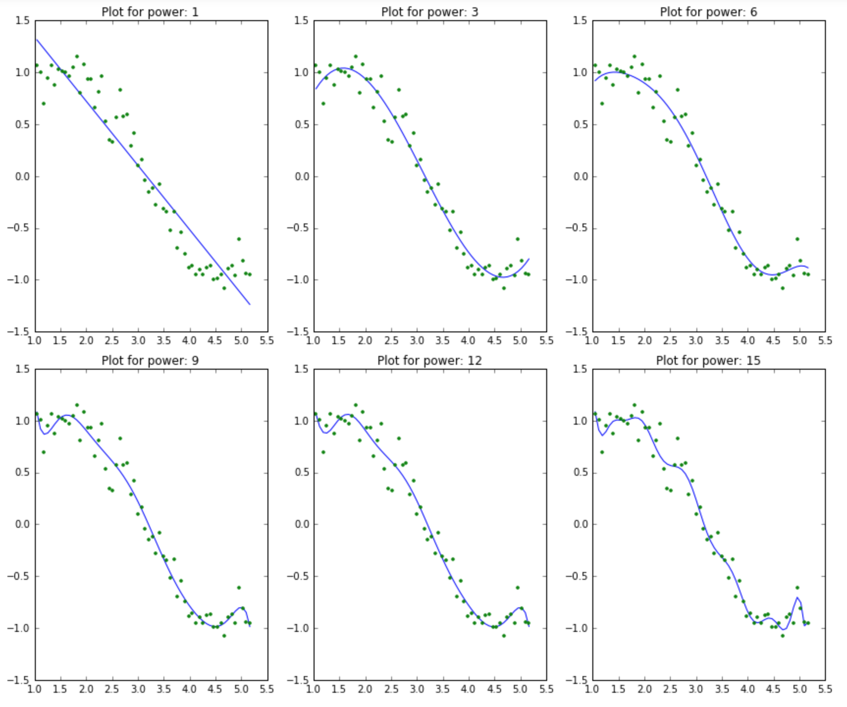
This clearly aligns with our initial understanding. As the model complexity increases, the models tend to fit even smaller deviations in the training data set. Though this leads to overfitting, let’s keep this issue aside for some time and come to our main objective, i.e., the impact on the magnitude of coefficients. This can be analyzed by looking at the data frame created above.
Python Code
#Set the display format to be scientific for ease of analysis
pd.options.display.float_format = '{:,.2g}'.format
coef_matrix_simple
The output looks like this:

It is clearly evident that the size of coefficients increases exponentially with an increase in model complexity. I hope this gives some intuition into why putting a constraint on the magnitude of coefficients can be a good idea to reduce model complexity.
Let’s try to understand this even better.
What does a large coefficient signify? It means that we’re putting a lot of emphasis on that feature, i.e., the particular feature is a good predictor for the outcome. When it becomes too large, the algorithm starts modeling intricate relations to estimate the output and ends up overfitting the particular training data.
I hope the concept is clear. Now, let’s understand ridge and lasso regression in detail and see how well they work for the same problem.
How Does Ridge Regression Work?
As mentioned before, ridge regression performs ‘L2 regularization‘, i.e., it adds a factor of the sum of squares of coefficients in the optimization objective. Thus, ridge regression optimizes the following:
Objective = RSS + α * (sum of the square of coefficients)
Here, α (alpha) is the parameter that balances the amount of emphasis given to minimizing RSS vs minimizing the sum of squares of coefficients. α can take various values:
- α = 0:
- The objective becomes the same as simple linear regression.
- We’ll get the same coefficients as simple linear regression.
- α = ∞:
- The coefficients will be zero. Why? Because of infinite weightage on the square of coefficients, anything less than zero will make the objective infinite.
- 0 < α < ∞:
- The magnitude of α will decide the weightage given to different parts of the objective.
- The coefficients will be somewhere between 0 and ones for simple linear regression.
I hope this gives some sense of how α would impact the magnitude of coefficients. One thing is for sure – any non-zero value would give values less than that of simple linear regression. By how much? We’ll find out soon. Leaving the mathematical details for later, let’s see ridge regression in action on the same problem as above.
Function for Ridge Regression
First, let’s define a generic function for ridge regression similar to the one defined for simple linear regression. The Python code is:
from sklearn.linear_model import Ridge
def ridge_regression(data, predictors, alpha, models_to_plot={}):
    #Fit the model
    ridgereg = Ridge(alpha=alpha,normalize=True)
    ridgereg.fit(data[predictors],data['y'])
    y_pred = ridgereg.predict(data[predictors])

    #Check if a plot is to be made for the entered alpha
    if alpha in models_to_plot:
        plt.subplot(models_to_plot[alpha])
        plt.tight_layout()
        plt.plot(data['x'],y_pred)
        plt.plot(data['x'],data['y'],'.')
        plt.title('Plot for alpha: %.3g'%alpha)

    #Return the result in pre-defined format
    rss = sum((y_pred-data['y'])**2)
    ret = [rss]
    ret.extend([ridgereg.intercept_])
    ret.extend(ridgereg.coef_)
    return ret
Note the ‘Ridge’ function used here. It takes ‘alpha’ as a parameter on initialization. Also, keep in mind that normalizing the inputs is generally a good idea in every type of regression and should be used in the case of ridge regression as well.
Now, let’s analyze the result of Ridge regression for 10 different values of α ranging from 1e-15 to 20. These values have been chosen so that we can easily analyze the trend with changes in values of α. These would, however, differ from case to case.
Note that each of these 10 models will contain all the 15 variables, and only the value of alpha would differ. This differs from the simple linear regression case, where each model had a subset of features.
Python Code
#Initialize predictors to be set of 15 powers of x
predictors=['x']
predictors.extend(['x_%d'%i for i in range(2,16)])

#Set the different values of alpha to be tested
alpha_ridge = [1e-15, 1e-10, 1e-8, 1e-4, 1e-3,1e-2, 1, 5, 10, 20]

#Initialize the dataframe for storing coefficients.
col = ['rss','intercept'] + ['coef_x_%d'%i for i in range(1,16)]
ind = ['alpha_%.2g'%alpha_ridge[i] for i in range(0,10)]
coef_matrix_ridge = pd.DataFrame(index=ind, columns=col)

models_to_plot = {1e-15:231, 1e-10:232, 1e-4:233, 1e-3:234, 1e-2:235, 5:236}
for i in range(10):
    coef_matrix_ridge.iloc[i,] = ridge_regression(data, predictors, alpha_ridge[i], models_to_plot)
This would generate the following plot: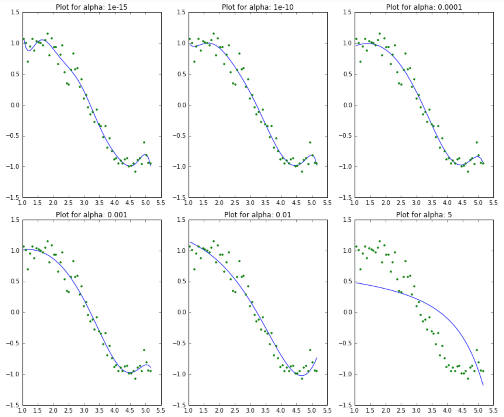
Here we can clearly observe that as the value of alpha increases, the model complexity reduces. Though higher values of alpha reduce overfitting, significantly high values can cause underfitting as well (e.g., alpha = 5). Thus alpha should be chosen wisely. A widely accepted technique is cross-validation, i.e., the value of alpha is iterated over a range of values, and the one giving a higher cross-validation score is chosen.
Let’s have a look at the value of coefficients in the above models:
Python Code
#Set the display format to be scientific for ease of analysis
pd.options.display.float_format = '{:,.2g}'.format
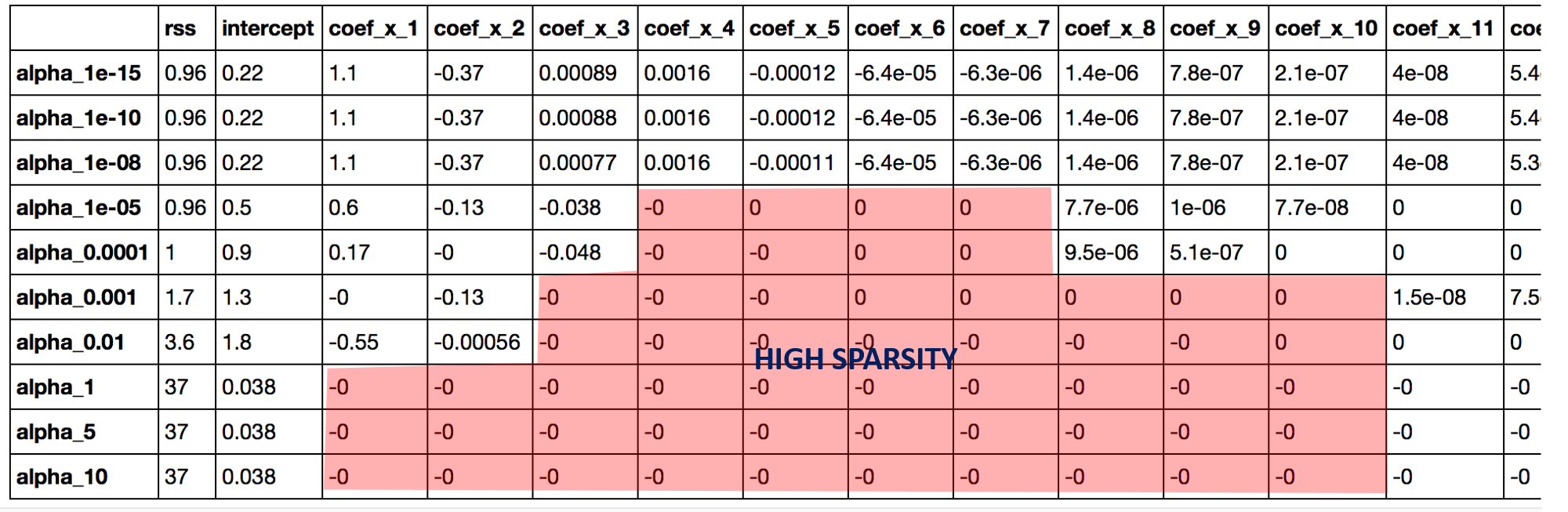
coef_matrix_ridgeThe table looks like: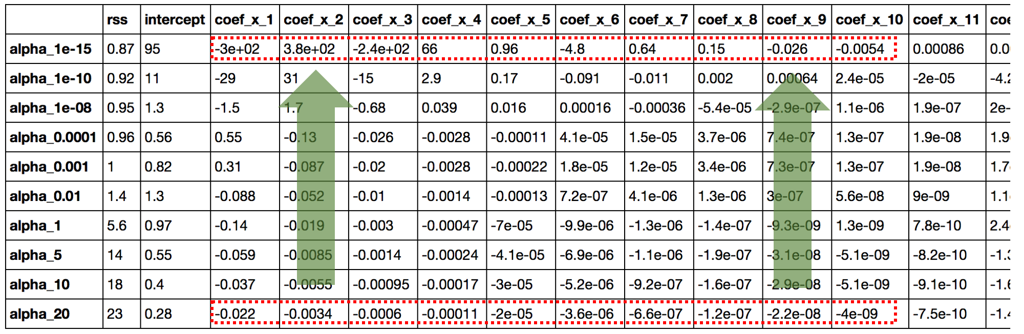
This straight away gives us the following inferences:
- The RSS increases with an increase in alpha.
- An alpha value as small as 1e-15 gives us a significant reduction in the magnitude of coefficients. How? Compare the coefficients in the first row of this table to the last row of the simple linear regression table.
- High alpha values can lead to significant underfitting. Note the rapid increase in RSS for values of alpha greater than 1
- Though the coefficients are really small, they are NOT zero.
The first 3 are very intuitive. But #4 is also a crucial observation. Let’s reconfirm the same by determining the number of zeros in each row of the coefficients data set:
Python Code
coef_matrix_ridge.apply(lambda x: sum(x.values==0),axis=1)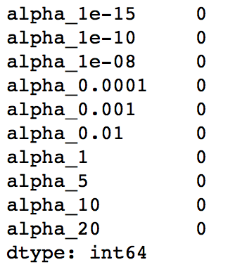
This confirms that all 15 coefficients are greater than zero in magnitude (can be +ve or -ve). Remember this observation and have a look again until it’s clear. This will play an important role later while comparing ridge with lasso regression.
How Does Lasso Regression Work?
LASSO stands for Least Absolute Shrinkage and Selection Operator. I know it doesn’t give much of an idea, but there are 2 keywords here – ‘absolute‘ and ‘selection. ‘
Let’s consider the former first and worry about the latter later.
Lasso regression performs L1 regularization, i.e., it adds a factor of the sum of the absolute value of coefficients in the optimization objective. Thus, lasso regression optimizes the following:
Objective = RSS + α * (sum of the absolute value of coefficients)
Here, α (alpha) works similar to that of the ridge and provides a trade-off between balancing RSS and the magnitude of coefficients. Like that of the ridge, α can take various values. Let’s iterate it here briefly:
- α = 0: Same coefficients as simple linear regression
- α = ∞: All coefficients zero (same logic as before)
- 0 < α < ∞: coefficients between 0 and that of simple linear regression
Defining Generic Function
Yes, its appearing to be very similar to Ridge till now. But hang on with me, and you’ll know the difference by the time we finish. Like before, let’s run lasso regression on the same problem as above. First, we’ll define a generic function:
from sklearn.linear_model import Lasso
def lasso_regression(data, predictors, alpha, models_to_plot={}):
    #Fit the model
    lassoreg = Lasso(alpha=alpha,normalize=True, max_iter=1e5)
    lassoreg.fit(data[predictors],data['y'])
    y_pred = lassoreg.predict(data[predictors])

    #Check if a plot is to be made for the entered alpha
    if alpha in models_to_plot:
        plt.subplot(models_to_plot[alpha])
        plt.tight_layout()
        plt.plot(data['x'],y_pred)
        plt.plot(data['x'],data['y'],'.')
        plt.title('Plot for alpha: %.3g'%alpha)

    #Return the result in pre-defined format
    rss = sum((y_pred-data['y'])**2)
    ret = [rss]
    ret.extend([lassoreg.intercept_])
    ret.extend(lassoreg.coef_)
    return ret
Notice the additional parameters defined in the Lasso function – ‘max_iter. ‘ This is the maximum number of iterations for which we want the model to run if it doesn’t converge before. This exists for Ridge as well, but setting this to a higher than default value was required in this case. Why? I’ll come to this in the next section.
Different Values of Alpha
Let’s check the output for 10 different values of alpha using the following code:
#Initialize predictors to all 15 powers of x
predictors=['x']
predictors.extend(['x_%d'%i for i in range(2,16)])

#Define the alpha values to test
alpha_lasso = [1e-15, 1e-10, 1e-8, 1e-5,1e-4, 1e-3,1e-2, 1, 5, 10]

#Initialize the dataframe to store coefficients
col = ['rss','intercept'] + ['coef_x_%d'%i for i in range(1,16)]
ind = ['alpha_%.2g'%alpha_lasso[i] for i in range(0,10)]
coef_matrix_lasso = pd.DataFrame(index=ind, columns=col)

#Define the models to plot
models_to_plot = {1e-10:231, 1e-5:232,1e-4:233, 1e-3:234, 1e-2:235, 1:236}

#Iterate over the 10 alpha values:
for i in range(10):
    coef_matrix_lasso.iloc[i,] = lasso_regression(data, predictors, alpha_lasso[i], models_to_plot)
This gives us the following plots: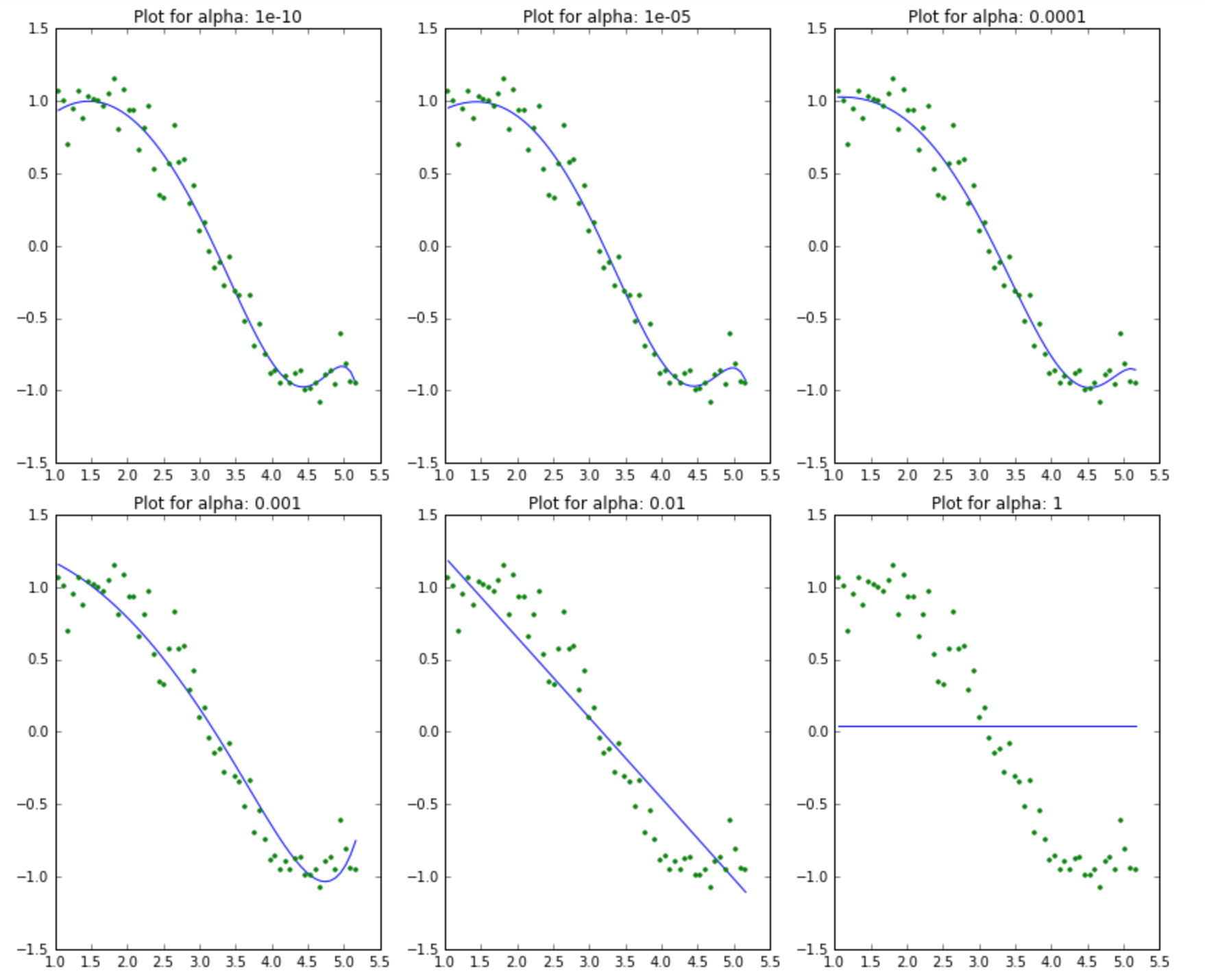
This again tells us that the model complexity decreases with an increase in the values of alpha. But notice the straight line at alpha=1. Appears a bit strange to me. Let’s explore this further by looking at the coefficients:
Apart from the expected inference of higher RSS for higher alphas, we can see the following:
- For the same values of alpha, the coefficients of lasso regression are much smaller than that of ridge regression (compare row 1 of the 2 tables).
- For the same alpha, lasso has higher RSS (poorer fit) as compared to ridge regression.
- Many of the coefficients are zero, even for very small values of alpha.
Inferences #1 and 2 might not always generalize but will hold for many cases. The real difference from the ridge is coming out in the last inference. Let’s check the number of coefficients that are zero in each model using the following code:
coef_matrix_lasso.apply(lambda x: sum(x.values==0),axis=1)Output:
We can observe that even for a small value of alpha, a significant number of coefficients are zero. This also explains the horizontal line fit for alpha=1 in the lasso plots; it’s just a baseline model! This phenomenon of most of the coefficients being zero is called ‘sparsity. ‘ Although lasso performs feature selection, this level of sparsity is achieved in special cases only, which we’ll discuss towards the end.
This has some really interesting implications on the use cases of lasso regression as compared to that of ridge regression. But before coming to the final comparison, let’s take a bird’s eye view of the mathematics behind why coefficients are zero in the case of lasso but not ridge.
Python Code
Some Underlying Mathematical Principles
Here’s a sneak peek into some of the underlying mathematical principles of regression. If you wish to get into the details, I recommend taking a good statistics textbook, like Elements of Statistical Learning.
Let’s start by reviewing the basic structure of data in a regression problem.
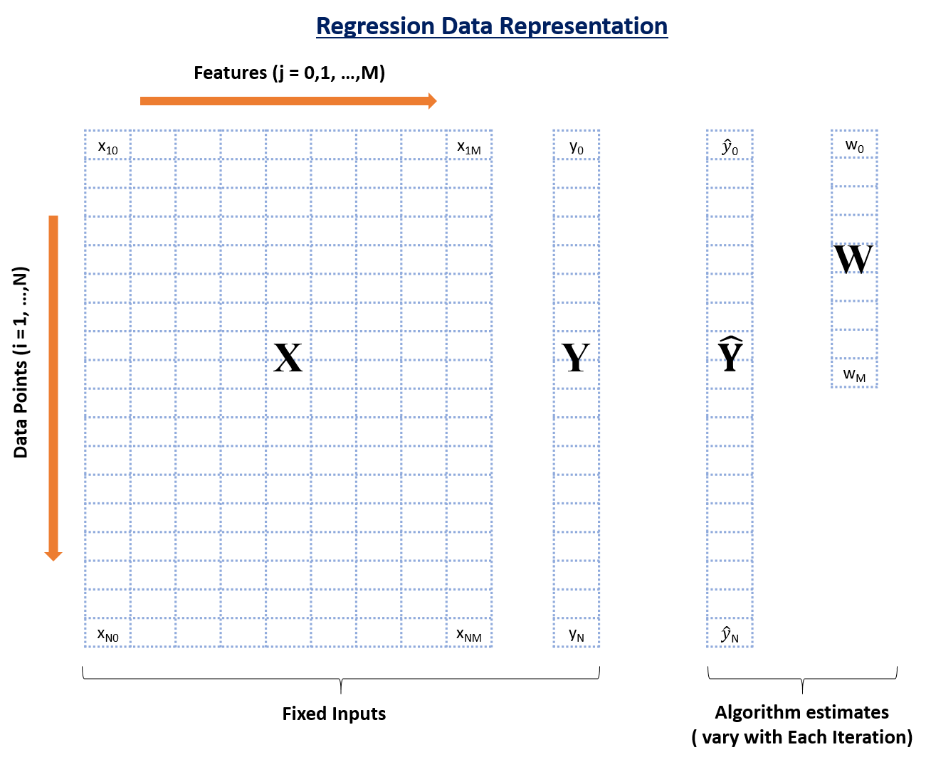
In this infographic, you can see there are 4 data elements:
- X: the matrix of input features (nrow: N, ncol: M+1)
- Y: the actual outcome variable (length:N)
- Yhat: these are predicted values of Y (length:N)
- W: the weights or the coefficients (length: M+1)
Here, N is the total number of data points available, and M is the total number of features. X has M+1 columns because of M features and 1 intercept.
The predicted outcome for any data point i is:

It is simply the weighted sum of each data point with coefficients as the weights. This prediction is achieved by finding the optimum value of weights based on certain criteria, which depends on the type of regression algorithm being used. Let’s consider all 3 cases:
Simple Linear Regression
The objective function (also called the cost) to be minimized is just the RSS (Residual Sum of Squares), i.e., the sum of squared errors of the predicted outcome as compared to the actual outcome. This can be depicted mathematically as:

In order to minimize this cost, we generally use a ‘gradient descent’ algorithm. The overall algorithm works like this:
1. initialize weights (say w=0)
2. iterate till not converged
   2.1 iterate over all features (j=0,1...M)
       2.1.1 determine the gradient
       2.1.2 update the jth weight by subtracting learning rate times the gradient
             w(t+1) = w(t) - learning rate * gradient
Here the important step is #2.1.1, where we compute the gradient. A gradient is nothing but a partial differential of the cost with respect to a particular weight (denoted as wj). The gradient for the jth weight will be:

This is formed from 2 parts:
- 2*{..}: This is formed because we’ve differentiated the square of the term in {..}
- -wj: This is the differentiation of the part in {..} wrt wj. Since it’s a summation, all others would become 0, and only wj would remain.
Step #2.1.2 involves updating the weights using the gradient. This updating step for simple linear regression looks like this:

Note the +ve sign in the RHS is formed after the multiplication of 2 -ve signs. I would like to explain point #2 of the gradient descent algorithm mentioned above, ‘iterate till not converged.‘ Here convergence refers to attaining the optimum solution within the pre-defined limit.
It is checked using the value of the gradient. If the gradient is small enough, it means we are very close to the optimum, and further iterations won’t substantially impact the coefficients. The lower limit on the gradient can be changed using the ‘tol‘ parameter.
Let’s consider the case of ridge regression now.
Ridge Regression
The objective function (also called the cost) to be minimized is the RSS plus the sum of squares of the magnitude of weights. This can be depicted mathematically as:

In this case, the gradient would be:

Again in the regularization part of a gradient, only wj remains, and all others would become zero. The corresponding update rule is:

Here we can see that the second part of the RHS is the same as that of simple linear regression. Thus, ridge regression is equivalent to reducing the weight by a factor of (1-2λη) first and then applying the same update rule as simple linear regression. I hope this explains why the coefficients get reduced to small numbers but never become zero.
Note that the criteria for convergence, in this case, remains similar to simple linear regression, i.e., checking the value of gradients. Let’s discuss Lasso regression now.
Lasso Regression
The objective function (also called the cost) to be minimized is the RSS plus the sum of the absolute value of the magnitude of weights. This can be depicted mathematically as:

In this case, the gradient is not defined as the absolute function is not differentiable at x=0. This can be illustrated as:
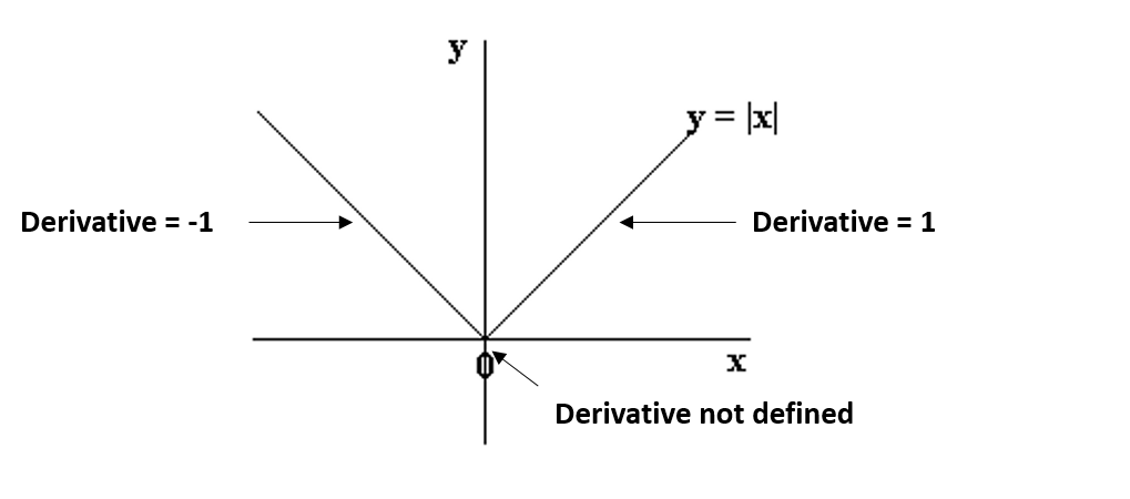
We can see that the parts on the left and right sides of 0 are straight lines with defined derivates, but the function can’t be differentiated at x=0. In this case, we have to use a different technique called coordinate descent, which is based on the concept of sub-gradients. One of the coordinate descent follows the following algorithms (this is also the default in sklearn):
1. initialize weights (say w=0)
2. iterate till not converged
   2.1 iterate over all features (j=0,1...M)
       2.1.1 update the jth weight with a value which minimizes the cost
#2.1.1 might look too generalized. But I’m intentionally leaving the details and jumping to the update rule:

Sample Project to Apply Your Regression Skills
Problem Statement
Demand forecasting is a key component of every growing online business. Without proper demand forecasting processes in place, it can be nearly impossible to have the right amount of stock on hand at any given time. A food delivery service has to deal with a lot of perishable raw materials, which makes it all the more important for such a company to accurately forecast daily and weekly demand.
Too much inventory in the warehouse means more risk of wastage, and not enough could lead to out-of-stocks — and push customers to seek solutions from your competitors. In this challenge, get a taste of the demand forecasting challenge using a real dataset.
Difference Between Actual and Predicted Outcome
Here g(w-j) represents (but not exactly) the difference between the actual outcome and the predicted outcome considering all EXCEPT the jth variable. If this value is small, it means that the algorithm is able to predict the outcome fairly well even without the jth variable, and thus it can be removed from the equation by setting a zero coefficient. This gives us some intuition into why the coefficients become zero in the case of lasso regression.
In coordinate descent, checking convergence is another issue. Since gradients are not defined, we need an alternate method. Many alternatives exist, but the simplest one is to check the step size of the algorithm. We can check the maximum difference in weights in any particular cycle overall feature weights (#2.1 of the algorithm above).
If this is lower than the specified ‘tol,’ the algorithm will stop. The convergence is not as fast as the gradient descent. If a warning appears saying that the algorithm stopped before convergence, we might have to set the ‘max_iter’ parameter. This is why I specified this parameter in the Lasso generic function.
Let’s summarize our understanding by comparing the coefficients in all the three cases using the following visual, which shows how the ridge and lasso coefficients behave in comparison to the simple linear regression case.
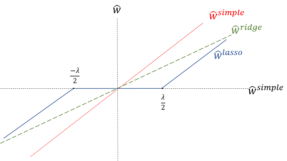
Reinforced Facts
Apologies for the lack of visual appeal. But I think it is good enough to re-inforced the following facts:
- The ridge coefficients are a reduced factor of the simple linear regression coefficients and thus never attain zero values but very small values.
- The lasso coefficients become zero in a certain range and are reduced by a constant factor, which explains their low magnitude in comparison to the ridge.
Before going further, one important issue in the case of both ridge and lasso regression is intercept handling. Generally, regularizing the intercept is not a good idea and should be left out of regularization. This requires slight changes in the implementation, which I’ll leave you to explore.
Comparison Between Ridge Regression and Lasso Regression
Now that we have a fair idea of how ridge and lasso regression work, let’s try to consolidate our understanding by comparing them and appreciating their specific use cases. I will also compare them with some alternate approaches. Let’s analyze these under three buckets:
Key Difference
- Ridge: It includes all (or none) of the features in the model. Thus, the major advantage of ridge regression is coefficient shrinkage and reducing model complexity.
- Lasso: Along with shrinking coefficients, the lasso also performs feature selection. (Remember the ‘selection‘ in the lasso full-form?) As we observed earlier, some of the coefficients become exactly zero, which is equivalent to the particular feature being excluded from the model.
Traditionally, techniques like stepwise regression were used to perform feature selection and make parsimonious models. But with advancements in Machine-Learning, ridge and lasso regressions provide very good alternatives as they give much better output, require fewer tuning parameters, and can be automated to a large extent.
Typical Use Cases
- Ridge: It is majorly used to prevent overfitting. Since it includes all the features, it is not very useful in the case of exorbitantly high #features, say in millions, as it will pose computational challenges.
- Lasso: Since it provides sparse solutions, it is generally the model of choice (or some variant of this concept) for modeling cases where the #features are in millions or more. In such a case, getting a sparse solution is of great computational advantage as the features with zero coefficients can be ignored.
It’s not hard to see why the stepwise selection techniques become practically cumbersome to implement in high-dimensionality cases. Thus, the lasso provides a significant advantage.
Presence of Highly Correlated Features
- Ridge: It generally works well even in the presence of highly correlated features, as it will include all of them in the model. Still, the coefficients will be distributed among them depending on the correlation.
- Lasso: It arbitrarily selects any feature among the highly correlated ones and reduces the coefficients of the rest to zero. Also, the chosen variable changes randomly with changes in model parameters. This generally doesn’t work that well as compared to ridge regression.
This disadvantage of the lasso can be observed in the example we discussed above. Since we used a polynomial regression, the variables were highly correlated. (Not sure why? Check the output of data.corr() ). Thus, we saw that even small values of alpha were giving significant sparsity (i.e., high #coefficients as zero).
Along with Ridge and Lasso, Elastic Net is another useful technique that combines both L1 and L2 regularization. It can be used to balance out the pros and cons of ridge and lasso regression. I encourage you to explore it further.
Conclusion
In this article, we got an overview of regularization using ridge and lasso regression. We then found out why penalizing the magnitude of coefficients should give us parsimonious models. Next, we went into details of ridge and lasso regression and saw their advantages over simple linear regression. We also understood how and why they should work. We also peeked into the mathematical part of the regressions.
Regularization techniques are really useful, and I encourage you to implement them. If you’re ready to take the challenge, you must try them on the BigMart Sales Prediction problem discussed at the beginning of this article.
Key Takeaways
- Ridge and Lasso Regression are regularization techniques used to prevent overfitting in linear regression models by adding a penalty term to the loss function.
- In Python, scikit-learn provides easy-to-use functions for implementing Ridge and Lasso regression with hyperparameter tuning and cross-validation.
- Ridge regression can handle multicollinearity in the input data by reducing the impact of correlated features on the coefficients, while Lasso regression automatically selects the most important features for prediction.
Frequently Asked Questions
A. Ridge and Lasso Regression are regularization techniques in machine learning. Ridge adds L2 regularization, and Lasso adds L1 to linear regression models, preventing overfitting.
A. Use Ridge when you have many correlated predictors and want to avoid multicollinearity. Use Lasso when feature selection is crucial or when you want a sparse model.
A. Ridge Regression adds a penalty term proportional to the square of the coefficients, while Lasso adds a penalty term proportional to the absolute value of the coefficients, which can lead to variable selection.
A. Ridge and Lasso are used to prevent overfitting in regression models by adding regularization terms to the cost function, encouraging simpler models with fewer predictors and more generalizability.
Aarshay graduated from MS in Data Science at Columbia University in 2017 and is currently an ML Engineer at Spotify New York. He works at an intersection or applied research and engineering while designing ML solutions to move product metrics in the required direction. He specializes in designing ML system architecture, developing offline models and deploying them in production for both batch and real time prediction use cases.


Good read, liked the way you explained why weight constraining is essential for regularization. Can you also perform the same experiments on Elastic Net and update this blog?
Hi Nilabhra, Thanks for reaching out. Yes it would be a good idea to discuss Elastic Net but I'll probably take this up in a separate article. I suppose there is sufficient content here to digest and I can discuss Elastic Net along with other regression techniques in future. Stay tuned! Cheers!
Beautiful, I will like this article ported to R please (I am somehow more happy in R than python)
Thanks for reaching out. I'll try to put together the R codes and revert back to you in about a week's time.
Hello Dr. Samuel, My apologies for not being able to stand upto my commitment for delivering the R-codes. I'm a bit crunched for bandwidth but I have this in the pipeline. Not sure when I'll be able to come back. If you have any juniors working under you on this, please feel free to ask them to reach to me for help through our discussion portal. Thank you!
Hi, It was a good post detailing the Ridge and Lasso regression. Great effort. However, it could have been complete, had the concept of multicollinearity been discussed in the context of Ridge regression. This is because to address this ticklish issue of multicollinearity, we have two alternative remedies in the form of ridge regression and principal component regression. Bests
Hello professor, Thanks for your valuable feedback. I suppose it'll be better if I discuss multi-collinearity in a separate article. You can expect it in future. Please stay tuned! Cheers!
You are an excellent teacher my friend, keep up the good work!
Thanks! I'll try my best..
Excellent write-up Aarshay. Deeply appreciate.
Thanks Tuhin!
Awesome arshay..keep up the learning and good work
For sure :)
Informative article. I understand LASSO shrunk coefficients to zero. Just wondering, after shrinkage, can any coefficient regain value. If yes, under what conditions it may happen so., Thanks.
I believe it can regain value. Actually it should depend on the selection of feature (step #2.1) in coordinate descent algorithm. Step #2.1 says that the algo will cycle through all features and optimize for one particular feature at a time. So, it might be possible that a non-zero optimum value exist in a future iteration which will cause the weight to regain value. It might be helpful to look into the contour plots of coordinate descent steps. There you can observe that it works in steps with a step along one particular dimension (in terms of weights) at a time. So a step in one direction can result in the algorithm choosing a non-zero step in another dimension even though it choose a zero step for the same dimension earlier. It might not be very intuitive but its possible. I have observed this happening. If we don’t want this to happen. We can use a different method to select the feature to optimize in step#2.1. For instance, we might set a rule that once a feature becomes zero, it will not be selected. Hope this helps.
Hello, really good and illustrative article. Gives a good impression of ridge and Lasso regression and definitely very helpful. Keep up the good work! p.s. Just two small corrections: 1) a $lambda$ got lost in the second line of the cost function for ridge regression. 2) I think that $w_j$ in the associated gradient expression of the cost function should be replaced by $x_ij$ and the whole expression multiplied by (-2)
Hi Tim, I'm glad you liked it. :) And thanks for pointing out the typing errors. I've updated the same. Cheers!
Really a nice article to understand lasso and ridge regression. However here in this article why are you reffering to simple linear regression instead of multiple linear regression. Any specific reason?
Thanks :) I'm sorry I didn't get you simple linear regression point. I've used a polynomial regression example here with 15 variables. Please elaborate.
I mean to say that you were comparing ridge and lasso model coefficients with simple linear regression coefficients. I.e you have mentioned (Compare the coefficients in the first row of this table to the last row of simple linear regression table.) ...Nothing wrong but it's just to correct my understanding.
My bad. I used an incorrect term. By 'simple' here I meant the regression without regularization and not the 'simple' in terms of single variable. Thanks for reaching out and for reading this in such depth. Please feel free to reach out in case you face any other challenges :)
When writing the formula for #2.1.1, why did you introduce `k` and not just use `j`?
i'm sorry I didn't get which part are you referring to.
Is the equation for predicted value of linear correction correct? (http://i1.wp.com/www.analyticsvidhya.com/wp-content/uploads/2016/01/eq1.png) Should there not be a bias added that is not multiplied by the weight?
Here 'j' is starting with 0. So the bias term is included in matrix for easy vectorization of calculation. The weight should be 1 always.
Hello, How to calculate lambda(max) for any model? I am running in loop many humdred models for the same Lasso code. If I specify a static range of lambda and apply cross validation, it throws me very less number of features for some models while so many for other models. I want to calculate lambda(max) for each model then specify the range of lambda based on that and do cross validation to get appropriate number of features. My intention is feature selection here. I am using python.
I'm not sure if I understood your concern currently. I'll explain a strategy which I would use to select the best value of lambda. First you should check for say 10 values which are separated by a good margin, say 1e-15, 1e-12, 1e-9 and so on upto say 1e5 or so. Once you do cross-validation on these, you'll get a sense of the range in which optimum value will lie. Then you can go for closer values in that range. Talking about the #features, you should choose the model with best CV score. If you think its not making sense, you should also try a higher number of folds and check the variance of error in different folds and not just the mean error. Hope this helps.
Refer Lasso regression , am using py 3.5, I changed the value of max_iter to 1e7, even then am getting a ConvergenceWarning that Objective did not converge. You might want to increase the number of iterations. Will appreciate if you can throw some light on this....
This might happen for some of the alpha values. If you read carefully, I have mentioned this towards the end of the lasso section. Some alpha values can result in a poor fit and thus the least square objective will not converge to the minimum value. One solution is to choose higher #iterations but if the problem persists for even high values, you should consider leaving that specific alpha value. Note that the alpha values causing this will vary from case to case and you should not keep any universal values of alpha in your mind. Hope this helps.
Thanks for the article, this was very helpful. One point is a little unclear to me, however. I can see that the lasso regression will produce zero values where ridge regression will likely produce just small weights. However, it is unclear to me whether this is a result of the differently defined cost function or of the different minimization algorithm implemented. I understand that lasso, as you explained, forces the use of coordinate descent rather than gradient descent, since the gradient is undefined. But, couldn't you use coordinate descent with ridge regression? And would that not produce zeros at a higher rate than gradient descent? Also, the function g(w_j) is a little mysterious to me.
I think you're getting mixed up here. Coordinate descent is not something applied by choice. The contour plot in case of lasso regression is such that coordinate descent has to be applied. That's not the case for ridge. If you go a little deeper into the mathematics, you'll understand better. There's a Machine Learning specialization on coursera which you can check out if you're interested in digging deeper! Hope this helps..
Excellent piece of work my friend. Please publish more.
Thanks a lot Aarshay for this excellent tutorial. Now I understand better why I should use LASSO instead of forward stepwise regression for shrinking an ODE system.
Hello, Thanks for your article, very useful. Not sure if it's a mistake but, on the graph showing the comparison between simple linear, Lasso and Ridge regression. you labeled the x-axis as "w simple", whereas "w simple" is already labeled for the red line. Should the x-axis not be labeled as "lambda" ?
Perfect and clear. Thanks a lot
Hi, Thanks for sharing. I am wondering how to formulate g(w-j) in Lasso regression here. Could you please provide some information? Many thanks!
Thanks for making it easy to understand!
Hi Aarshay, I have a couple of questions w.r.t. regularized regression (Lasso & Ridge). Hope you could answer them 1.) In unregularized regression, we use adjusted R2. Similarly, what are the model evaluation parameters that we can use for regularized models ? 2.) Basically, regularized model is min( error term + regularization term). So in this case, will Mean Square Error (MSE) for regularized models will always be higher than that of unregularized model ?
Great article...helped me a lot !!
Hello Aarshay Jain, Really a nice stuff . Thank you for sharing .
Hello! great work! One question on leaving the intercept out ; how does this work in R? For example when I run cv.clmnet I use the 1 standard error validated values. When I predict using the coefficients the intercept has been changed a little bit. Any advice would be greatly appreciated, thanks!
Thank you for clarification about regularized regression model.
This article is great! I learnt a lot from it! Thank You!!!
Excellent write up. appreciate that. How can I add the CI of the coefficients to the summary report though?
thanks for the great article. I was wondering as to how would you suggest I iterate the alpha values so that at the end result we may be able to arrive to the right regression equation? Will it be good to start with 1e-10 and then 1e+10 and then observe the RSS value and then reduce the next alphas in between the range until the RSS reduces?
Very nice and clear article. Well done.
1.. What kind of predictors can be used with Lasso? 2. If categorical predictors can be used, should they be re-coded to have numerical values? ex: yes/no values re-coded to be 1/0 3. Can categorical variables such as location (U(urban)/R(rural)) be used without any conversion/re-coding?
sir i m in great trouble. i have to submit my synopses. i m working on the field of predcition. i have predicted my data set by NARNET. now inst has given me a task to compare my result with lasso,ridge and svr. but i have no idea about the predciction by these methods.can u plz help me regarding this. plz sir i m with a lot of hope. my entire carrier is depending upon this. plz sir thanks srikanta
sir i m in great trouble. i have to submit my synopses. i m working on the field of predcition. i have predicted my data set by NARNET. now inst has given me a task to compare my result with lasso,ridge and svr. but i have no idea about the predciction by these methods.can u plz help me regarding this. plz sir i m with a lot of hope. my entire carrier is depending upon this. plz sir. plz anybody can help [email protected] thanks srikanta
Excellent read, excellent explanation even of the maths. Keep up the good work!
Super thanks !
such a great article! thanks
"It is clearly evident that the size of coefficients increase exponentially with increase in model complexity. I hope this gives some intuition into why putting a constraint on the magnitude of coefficients can be a good idea to reduce model complexity." This above statement cleared my whole doubt. Nice writeup. Cheers!
Hi Mohammed, Glad you found this helpful! Happy learning!
Thanks ever so much for your explanation
Hello, that url "http://statweb.stanford.edu/~tibs/ElemStatLearn/" can not open.
Hi, Thank you for pointing it out. We have updated the same in the article.
Great Article.. Gave a clear understanding to the concept of Regularization with practical examples.
Hi Aarshay, Great blog and many thanks for such explanations on lasso and ridge. However, I am facing a problem when trying to do the same. When I try the lasso, with exactly the same "data" as you, and exactly the same parameters and same alpha values as well, I systemacilly get a "non convergence error". I really do not understand why, since, apparently, you did not face such a problem while you did it yourself. Any help would be appreciated. Thank you on beforehand.
An extremely interesting article... very precise, complete and intuitive! Really thanks!
Well explanatory, keep up the good work.
Wow Aarshay what an impressively pedagogical post. You are an excellent teacher. I am currently struggling with a problem that had a lot of raw data (about 2500 features and about 1e10 observations). I don’t have a way to treat that amount of data so I am only using (monthly) covariance matrices. I would like to do a Lasso regularisation on those, as opposed to raw data. There is a package in Python that does this (Glasso) but it’s quite intricate and I am struggling to find any clear user guide or example. Do you think you could do a post on that subject?