How to Use Multinomial and Ordinal Logistic Regression in R?
Introduction
Most of us have limited knowledge of regression. Of these, linear and logistic regression are our favorite ones. As an interesting fact, regression has extended capabilities to deal with different types of variables. Do you know, that regression has provisions for dealing with multi-level dependent variables too? I’m sure, you didn’t. Neither did I until I explored this aspect of Regression.
For multi-level dependent variables, there are many machine learning algorithms that can do the job for you; such as naive Bayes, decision trees, random forests, etc. For starters, these algorithms can be a bit difficult to understand. But, if you very well understand logistic regression, mastering this new aspect of regression should be easy for you!
In this article, I’ve explained the method of using multinomial and ordinal regression. Also, for practical purposes, I’ve demonstrated this algorithm in a step-wise fashion in R. This article draws inspiration from a detailed article here. I have added my own take on it.
Note: This article best suits R users having prior knowledge of logistic regression. However, if you use Python, you can still get an overall understanding of this regression method.

Table of Contents
What is Multinomial Logistic Regression?
Multinomial Logistic Regression (MLR) is a form of linear regression analysis conducted when the dependent variable is nominal with more than two levels. It helps to describe data and explain the relationship between one dependent nominal variable and one or more continuous-level (interval or ratio scale) independent variables. You can understand a nominal variable as, a variable that has no intrinsic ordering.
For example, Types of Forests: ‘Evergreen Forest’, ‘Deciduous Forest’, ‘Rain Forest’
As you see, there is no intrinsic order in them, but each forest represents a unique category. In other words, multinomial regression is an extension of logistic regression, which analyzes dichotomous (binary) dependents.
How Does Multinomial Logistic Regression Work?
The multinomial logistic regression estimates a separate binary logistic regression model for each dummy variable. The result is M-1 binary logistic regression models. Each model conveys the effect of predictors on the probability of success in that category, in comparison to the reference category.
Each model has its own intercept and regression coefficients—the predictors can affect each category differently. Let’s compare this part with our classics – Linear and Logistic Regression.
Standard linear regression requires the dependent variable to be of continuous-level (interval or ratio) scale. However, logistic regression jumps the gap by assuming that the dependent variable is a stochastic event. The dependent variable describes the outcome of this stochastic event with a density function (a function of cumulated probabilities ranging from 0 to 1).
Statisticians then argue one event happens if the probability is less than 0.5 and the opposite event happens when the probability is greater than 0.5.
Now we know that MLR extends the binary logistic model to a model with numerous categories (in dependent variable). However, it has one limitation. The category to which an outcome belongs does not assume any order in it. For example, if we have N categories, all have an equal probability. In reality, we come across problems where categories have a natural order.
So, what to do when we have a natural order in categories of dependent variables? In such a situation, Ordinal Regression comes to our rescue.
What is Ordinal Logistic Regression?
Ordinal Regression (also known as Ordinal Logistic Regression) is another extension of binomial logistics regression. Ordinal regression helps in predicting the dependent variable with ‘ordered’ multiple categories and independent variables. In other words, it helps to facilitate the interaction of dependent variables (having multiple ordered levels) with one or more independent variables.
For example: Let us assume a survey is done. We asked a question to respondent where their answer lies between agree or disagree. The responses thus collected didn’t help us to generalize well. Later, we added levels to our responses such as Strongly Disagree, Disagree, Agree, Strongly Agree.
This helped us to observe a natural order in the categories. For our regression model to be realistic, we must appreciate this order instead of being naive to it, as in the case of MLR. Ordinal Logistic Regression addresses this fact. Ordinal means the order of the categories.
Examples of Logistic Regression
Before we perform this algorithm in R, let’s ensure that we have gained a concrete understanding using the cases below:
Case 1: Multinomial Regression
The modeling of program choices made by high school students can be done using Multinomial logit. The program choices are general program, vocational program, and academic program. Using their writing score and socioeconomic status, we can model their choice.
Based on a variety of attributes such as social status, channel type, awards and accolades received by the students, gender, economic status, and how well they can read and write in the subjects given, we can predict the choice of the type of program. The choice of programs with multiple levels (unordered) is the dependent variable. This case suits using the Multinomial Logistic Regression technique.
Case 2: Ordinal Regression
A study looks at factors that influence the decision of whether to apply to graduate school. College juniors are asked if they are unlikely, somewhat likely, or very likely to apply to graduate school. Hence, our outcome variable has three categories i.e. unlikely, somewhat likely, and very likely.
Data on parental educational status, class of institution (private or state-run), and current GPA are also collected. The researchers have reason to believe that the “distances” between these three points are not equal. For example, the “distance” between “unlikely” and “somewhat likely” may be shorter than the distance between “somewhat likely” and “very likely”. In such a case, we’ll use Ordinal Regression.
Multinomial Logistic Regression (MLR) in R
Step 1: Read the file
> library("foreign")
> ml <- read.dta("http://www.ats.ucla.edu/stat/data/hsbdemo.dta")
Step 2: Re-level the data
We begin with re-leveling the data.
> head(ml)
## id female ses schtyp prog read write math science socst ## 1 45 female low public vocation 34 35 41 29 26 ## 2 108 male middle public general 34 33 41 36 36 ## 3 15 male high public vocation 39 39 44 26 42 ## 4 67 male low public vocation 37 37 42 33 32 ## 5 153 male middle public vocation 39 31 40 39 51 ## 6 51 female high public general 42 36 42 31 39 ## honors awards cid ## 1 not enrolled 0 1 ## 2 not enrolled 0 1 ## 3 not enrolled 0 1 ## 4 not enrolled 0 1 ## 5 not enrolled 0 1 ## 6 not enrolled 0 1
> ml$prog2 <- relevel(ml$prog, ref = "academic")
Step 3: Now we’ll execute a multinomial regression with two independent variables.
> library("nnet")
> test <- multinom(prog2 ~ ses + write, data = ml)
## # weights: 15 (8 variable)
## initial value 219.722458
## iter 10 value 179.982880
## final value 179.981726
## converged> summary(test)
## Call:
 ## multinom(formula = prog2 ~ ses + write, data = ml)
 ##
 ## Coefficients:
 ##          (Intercept)  sesmiddle    seshigh      write
 ## general     2.852198 -0.5332810 -1.1628226 -0.0579287
 ## vocation    5.218260  0.2913859 -0.9826649 -0.1136037
 ##
 ## Std. Errors:
 ##          (Intercept) sesmiddle   seshigh      write
 ## general     1.166441 0.4437323 0.5142196 0.02141097
 ## vocation    1.163552 0.4763739 0.5955665 0.02221996
 ##
 ## Residual Deviance: 359.9635
 ## AIC: 375.9635
Interpretation
1. Model execution output shows some iteration history and includes the final negative log-likelihood 179.981726. This value is multiplied by two as shown in the model summary as the Residual Deviance.
2. The summary output has a block of coefficients and another block of standard errors. Each block has one row of values corresponding to one model equation. In the block of coefficients, we see that the first row is being compared to prog = “general” to our baseline prog = “academic” and the second row to prog = “vocation” to our baseline prog = “academic”.
3. A one-unit increase in write decreases the log odds of being in general program vs. academic program by 0.0579
4. A one-unit increase in write decreases the log odds of being in a vocation program vs. an academic program by 0.1136
5. The log odds of being in a general program than in an academic program will decrease by 1.163 if moving from ses=”low” to ses=”high”.
6. On the other hand, Log odds of being in a general program than in an academic program will decrease by 0.5332 if moving from ses=”low” to ses=”middle”
7. The log odds of being in a vocation program vs. in an academic program will decrease by 0.983 if moving from ses=”low” to ses=”high”
8. The log odds of being in a vocation program vs. in an academic program will increase by 0.291 if moving from ses=”low” to ses=”middle”
Step 4: Now we’ll calculate the Z score and p-value for the variables in the model.
> z <- summary(test)$coefficients/summary(test)$standard.errors
> z
## (Intercept) sesmiddle seshigh write ## general 2.445214 -1.2018081 -2.261334 -2.705562 ## vocation 4.484769 0.6116747 -1.649967 -5.112689
> p <- (1 - pnorm(abs(z), 0, 1))*2
> p
## (Intercept) sesmiddle seshigh write ## general 0.0144766100 0.2294379 0.02373856 6.818902e-03 ## vocation 0.0000072993 0.5407530 0.09894976 3.176045e-07
> exp(coef(test))## (Intercept) sesmiddle seshigh write ## general 17.32582 0.5866769 0.3126026 0.9437172 ## vocation 184.61262 1.3382809 0.3743123 0.8926116
The P-value tells us that the variables are not significant. Now we’ll explore the entire data set, and analyze if we can remove any variables which do not add to model performance.
> names(ml)## [1] "id" "female" "ses" "schtyp" "prog" "read" "write" ## [8] "math" "science" "socst" "honors" "awards" "cid" "prog2"
> levels(ml$female)## [1] "male" "female"
> levels(ml$ses)
## [1] "low" "middle" "high"
> levels(ml$schtyp)## [1] "public" "private"
> levels(ml$honors)
## [1] "not enrolled" "enrolled"
Step 5: Let’s now build a multinomial model on the entire data set after removing id and prog variables.
> test <- multinom(prog2 ~ ., data = ml[,-c(1,5,13)])## # weights: 39 (24 variable) ## initial value 219.722458 ## iter 10 value 178.757016 ## iter 20 value 155.866327 ## iter 30 value 154.365307 ## final value 154.365305 ## converged
> summary(test)## Call: ## multinom(formula = prog2 ~ ., data = ml[, -c(1, 5, 13)]) ## ## Coefficients: ## (Intercept) femalefemale sesmiddle seshigh schtypprivate ## general 5.692368 0.1547445 -0.2809824 -0.9632924107 -0.5872049 ## vocation 9.839107 0.4076641 1.2246933 0.0008659972 -1.9089941 ## read write math science socst ## general -0.04421300 -0.05434029 -0.1001477 0.10397170 -0.02486526 ## vocation -0.04124332 -0.05149742 -0.1209839 0.06341246 -0.07012002 ## honorsenrolled awards ## general -0.5963679 0.26104317 ## vocation 1.0986972 -0.08573852 ## ## Std. Errors: ## (Intercept) femalefemale sesmiddle seshigh schtypprivate ## general 2.385383 0.4514339 0.5224132 0.5934146 0.5597181 ## vocation 2.566895 0.4993567 0.5764471 0.6885407 0.8313621 ## read write math science socst ## general 0.03076523 0.05109711 0.03514069 0.03153073 0.02697888 ## vocation 0.03451435 0.05358824 0.03902319 0.03252487 0.02912126 ## honorsenrolled awards ## general 0.8708913 0.2969302 ## vocation 0.9798571 0.3708768 ## ## Residual Deviance: 308.7306 ## AIC: 356.7306
Step 6: Let’s check for fitted values now.
> head(fitted(test))## academic general vocation ## 1 0.08952937 0.1811189 0.7293518 ## 2 0.05219222 0.1229310 0.8248768 ## 3 0.54704495 0.0849831 0.3679719 ## 4 0.17103536 0.2750466 0.5539180 ## 5 0.10014015 0.2191946 0.6806652 ## 6 0.27287474 0.1129348 0.6141905
Once we have built the model, we’ll use it for prediction.
Step 7: Let us create a new data set with different permutations and combinations.
> expanded=expand.grid(female=c("female", "male", "male", "male"), ses=c("low","low","middle", "high"), schtyp=c("public", "public", "private", "private"), read=c(20,50,60,70), write=c(23,45,55,65), math=c(30,46,76,54), science=c(25,45,68,51), socst=c(30, 35, 67, 61), honors=c("not enrolled", "not enrolled", "enrolled","not enrolled"), awards=c(0,0,3,0,6) )
> head(expanded)
## female ses schtyp read write math science socst honors awards ## 1 female low public 20 23 30 25 30 not enrolled 0 ## 2 male low public 20 23 30 25 30 not enrolled 0 ## 3 male low public 20 23 30 25 30 not enrolled 0 ## 4 male low public 20 23 30 25 30 not enrolled 0 ## 5 female low public 20 23 30 25 30 not enrolled 0 ## 6 male low public 20 23 30 25 30 not enrolled 0
> predicted=predict(test,expanded,type="probs")
> head(predicted)
## academic general vocation ## 1 0.01357216 0.1759060 0.8105219 ## 2 0.01929452 0.2142205 0.7664850 ## 3 0.01929452 0.2142205 0.7664850 ## 4 0.01929452 0.2142205 0.7664850 ## 5 0.01357216 0.1759060 0.8105219 ## 6 0.01929452 0.2142205 0.7664850
Step 8: Now, we’ll calculate the prediction values.
The parameter type=”probs”, specifies our interest in probabilities. To plot predicted probabilities for intuitive understanding, we add predicted probability values to data.
> bpp=cbind(expanded, predicted)Step 9: Now we’ll calculate the mean probabilities within each level of ses.
> by(bpp[,4:7], bpp$ses, colMeans)
## bpp$ses: low ## read write math science ## 50.00 47.00 51.50 47.25 ## -------------------------------------------------------- ## bpp$ses: middle ## read write math science ## 50.00 47.00 51.50 47.25 ## -------------------------------------------------------- ## bpp$ses: high ## read write math science ## 50.00 47.00 51.50 47.25
I’ve used the melt() function from the ‘reshape2’ package. It “melts” data with the purpose of each row being a unique id-variable combination.
> library("reshape2")## Warning: package 'reshape2' was built under R version 3.1.3> bpp2 = melt (bpp,id.vars=c("female", "ses","schtyp", "read","write","math","science","socst","honors", "awards"),value.name="probablity")> head(bpp2)
## female ses schtyp read write math science socst honors awards ## 1 female low public 20 23 30 25 30 not enrolled 0 ## 2 male low public 20 23 30 25 30 not enrolled 0 ## 3 male low public 20 23 30 25 30 not enrolled 0 ## 4 male low public 20 23 30 25 30 not enrolled 0 ## 5 female low public 20 23 30 25 30 not enrolled 0 ## 6 male low public 20 23 30 25 30 not enrolled 0 ## variable probablity ## 1 academic 0.01357216 ## 2 academic 0.01929452 ## 3 academic 0.01929452 ## 4 academic 0.01929452 ## 5 academic 0.01357216 ## 6 academic 0.01929452
Step 10: Now, we will be plotting graphs to explore the distribution of dependent variables vs independent variables, using ggplot() function.
In ggplot, the first parameter in this function is the data values to be plotted. The second part is where (aes()) binds variables to the x and y-axis. We tell the plotting function to draw a line using geom_line(). We are differentiating the school types by plotting them in different colors.
> library("ggplot2")> ggplot(bpp2, aes(x = write, y = probablity, colour = ses)) +
geom_line() + facet_grid(variable ~ ., scales="free")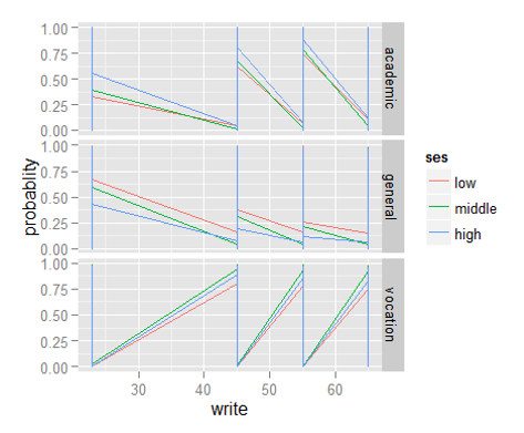
Till here, we have learned to use multinomial regression in R. As mentioned above, if you have prior knowledge of logistic regression, interpreting the results wouldn’t be too difficult. Let’s now proceed to understand ordinal regression in R.
Ordinal Logistic Regression (OLR) in R
Below are the steps to perform OLR in R:
Step 1: Load the Libraries
> require(foreign)
> require(ggplot2)
> require(MASS)
> require(Hmisc)
> require(reshape2)
Step 2: Load the data
> dat <- read.dta("http://www.ats.ucla.edu/stat/data/ologit.dta")> head(dat)
## apply pared public gpa ## 1 very likely 0 0 3.26 ## 2 somewhat likely 1 0 3.21 ## 3 unlikely 1 1 3.94 ## 4 somewhat likely 0 0 2.81 ## 5 somewhat likely 0 0 2.53 ## 6 unlikely 0 1 2.59
Let’s quickly understand the data.
The data set has a dependent variable known as apply. It has 3 levels namely “unlikely”, “somewhat likely”, and “very likely”, coded in 1, 2, and 3 respectively. 3 being highest and 1 being lowest. This situation is best for using ordinal regression because of the presence of ordered categories. Pared (0/1) refers to at least one parent who has a graduate degree; public (0/1) refers to the type of undergraduate institute.
For building this model, we will be using the polr command to estimate an ordered logistic regression. Then, we’ll specify Hess=TRUE to let the model output show the observed information matrix from optimization which is used to get standard errors.
> m <- polr(apply ~ pared + public + gpa, data = dat, Hess=TRUE)> summary(m)
## Call:
 ## polr(formula = apply ~ pared + public + gpa, data = dat, Hess = TRUE)
 ##
 ## Coefficients:
 ##           Value Std. Error t value
 ## pared   1.04769     0.2658  3.9418
 ## public -0.05879     0.2979 -0.1974
 ## gpa     0.61594     0.2606  2.3632
 ##
 ## Intercepts:
 ##                             Value   Std. Error t value
 ## unlikely|somewhat likely     2.2039  0.7795     2.8272
 ## somewhat likely|very likely  4.2994  0.8043     5.3453
 ##
 ## Residual Deviance: 717.0249
 ## AIC: 727.0249
We see the usual regression output coefficient table including the value of each coefficient, standard errors, t values, estimates for the two intercepts, residual deviance, and AIC. AIC is the information criteria. Lesser the better.
Step 3: Now we’ll calculate some essential metrics such as p-value, CI, Odds ratio
> ctable <- coef(summary(m))
## Value Std. Error t value ## pared 1.04769010 0.2657894 3.9418050 ## public -0.05878572 0.2978614 -0.1973593 ## gpa 0.61594057 0.2606340 2.3632399 ## unlikely|somewhat likely 2.20391473 0.7795455 2.8271792 ## somewhat likely|very likely 4.29936315 0.8043267 5.3452947
> p <- pnorm(abs(ctable[, "t value"]), lower.tail = FALSE) * 2> ctable <- cbind(ctable, "p value" = p)
## Value Std. Error t value p value ## pared 1.04769010 0.2657894 3.9418050 8.087072e-05 ## public -0.05878572 0.2978614 -0.1973593 8.435464e-01 ## gpa 0.61594057 0.2606340 2.3632399 1.811594e-02 ## unlikely|somewhat likely 2.20391473 0.7795455 2.8271792 4.696004e-03 ## somewhat likely|very likely 4.29936315 0.8043267 5.3452947 9.027008e-08
# confidence intervals> ci <- confint(m)
## Waiting for profiling to be done...
## 2.5 % 97.5 % ## pared 0.5281768 1.5721750 ## public -0.6522060 0.5191384 ## gpa 0.1076202 1.1309148
> exp(coef(m))
## pared public gpa ## 2.8510579 0.9429088 1.8513972
## OR and CI> exp(cbind(OR = coef(m), ci))
## OR 2.5 % 97.5 % ## pared 2.8510579 1.6958376 4.817114 ## public 0.9429088 0.5208954 1.680579 ## gpa 1.8513972 1.1136247 3.098490
Interpretation
1. One unit increase in parental education, from 0 (Low) to 1 (High), the odds of “very likely” applying versus “somewhat likely” or “unlikely” applying combined are 2.85 greater.
2. The odds of “very likely” or “somewhat likely” applying versus “unlikely” applying is 2.85 times greater.
3. For GPA, when a student’s GPA moves 1 unit, the odds of moving from “unlikely” applying to “somewhat likely” or “very likely” applying (or from the lower and middle categories to the high category) are multiplied by 1.85.
Step 4: Let’s now try to enhance this model to obtain better prediction estimates.
> summary(m)
## Call:
## polr(formula = apply ~ pared + public + gpa, data = dat, Hess = TRUE)
##
## Coefficients:
## Value Std. Error t value
## pared 1.04769 0.2658 3.9418
## public -0.05879 0.2979 -0.1974
## gpa 0.61594 0.2606 2.3632
##
## Intercepts:
## Value Std. Error t value
## unlikely|somewhat likely 2.2039 0.7795 2.8272
## somewhat likely|very likely 4.2994 0.8043 5.3453
##
## Residual Deviance: 717.0249
## AIC: 727.0249> summary(update(m, method = "probit", Hess = TRUE), digits = 3)
## Call:
 ## polr(formula = apply ~ pared + public + gpa, data = dat, Hess = TRUE,
 ##     method = "probit")
 ##
 ## Coefficients:
 ##         Value Std. Error t value
 ## pared  0.5981      0.158  3.7888
 ## public 0.0102      0.173  0.0588
 ## gpa    0.3582      0.157  2.2848
 ##
 ## Intercepts:
 ##                             Value Std. Error t value
 ## unlikely|somewhat likely    1.297 0.468      2.774
 ## somewhat likely|very likely 2.503 0.477      5.252
 ##
 ## Residual Deviance: 717.4951
 ## AIC: 727.4951
> summary(update(m, method = "logistic", Hess = TRUE), digits = 3)
## Call:
 ## polr(formula = apply ~ pared + public + gpa, data = dat, Hess = TRUE,
 ##     method = "logistic")
 ##
 ## Coefficients:
 ##          Value Std. Error t value
 ## pared   1.0477      0.266   3.942
 ## public -0.0588      0.298  -0.197
 ## gpa     0.6159      0.261   2.363
 ##
 ## Intercepts:
 ##                             Value  Std. Error t value
 ## unlikely|somewhat likely     2.204  0.780      2.827
 ## somewhat likely|very likely  4.299  0.804      5.345
 ##
 ## Residual Deviance: 717.0249
 ## AIC: 727.0249
> summary(update(m, method = "cloglog", Hess = TRUE), digits = 3)
## Call:
 ## polr(formula = apply ~ pared + public + gpa, data = dat, Hess = TRUE,
 ##     method = "cloglog")
 ##
 ## Coefficients:
 ##        Value Std. Error t value
 ## pared  0.517      0.161   3.202
 ## public 0.108      0.168   0.643
 ## gpa    0.334      0.154   2.168
 ##
 ## Intercepts:
 ##                             Value Std. Error t value
 ## unlikely|somewhat likely    0.871 0.455      1.912
 ## somewhat likely|very likely 1.974 0.461      4.287
 ##
 ## Residual Deviance: 719.4982
 ## AIC: 729.4982
Step 5: Let’s add interaction terms here.
> head(predict(m, dat, type = “p”))
##    unlikely somewhat likely very likely
 ## 1 0.5488310       0.3593310  0.09183798
 ## 2 0.3055632       0.4759496  0.21848725
 ## 3 0.2293835       0.4781951  0.29242138
 ## 4 0.6161224       0.3126888  0.07118879
 ## 5 0.6560149       0.2833901  0.06059505
 ## 6 0.6609240       0.2797117  0.05936430
> addterm(m, ~.^2, test = "Chisq")
## Single term additions
 ##
 ## Model:
 ## apply ~ pared + public + gpa
 ##              Df    AIC     LRT Pr(Chi)
 ## <none>          727.02
 ## pared:public  1 727.81 1.21714  0.2699
 ## pared:gpa     1 728.98 0.04745  0.8276
 ## public:gpa    1 728.60 0.42953  0.5122
> m2 <- stepAIC(m, ~.^2)> m2
## Start:  AIC=727.02
 ## apply ~ pared + public + gpa
 ##
 ##                Df    AIC
 ## - public        1 725.06
 ## <none>            727.02
 ## + pared:public  1 727.81
 ## + public:gpa    1 728.60
 ## + pared:gpa     1 728.98
 ## - gpa           1 730.67
 ## - pared         1 740.60
 ##
 ## Step:  AIC=725.06
 ## apply ~ pared + gpa
 ##
 ##             Df    AIC
 ## <none>         725.06
 ## + pared:gpa  1 727.02
 ## + public     1 727.02
 ## - gpa        1 728.79
 ## - pared      1 738.60
> summary(m2)
## Call:
 ## polr(formula = apply ~ pared + gpa, data = dat, Hess = TRUE)
 ##
 ## Coefficients:
 ##        Value Std. Error t value
 ## pared 1.0457     0.2656   3.937
 ## gpa   0.6042     0.2539   2.379
 ##
 ## Intercepts:
 ##                             Value  Std. Error t value
 ## unlikely|somewhat likely    2.1763 0.7671     2.8370
 ## somewhat likely|very likely 4.2716 0.7922     5.3924
 ##
 ## Residual Deviance: 717.0638
 ## AIC: 725.0638
> m2$anova
## Stepwise Model Path
 ## Analysis of Deviance Table
 ##
 ## Initial Model:
 ## apply ~ pared + public + gpa
 ##
 ## Final Model:
 ## apply ~ pared + gpa
 ##
 ##
 ##       Step Df   Deviance Resid. Df Resid. Dev      AIC
 ## 1                              395   717.0249 727.0249
 ## 2 - public  1 0.03891634       396   717.0638 725.0638
> anova(m, m2)
## Likelihood ratio tests of ordinal regression models
 ##
 ## Response: apply
 ##                  Model Resid. df Resid. Dev   Test    Df   LR stat.
 ## 1          pared + gpa       396   717.0638
 ## 2 pared + public + gpa       395   717.0249 1 vs 2     1 0.03891634
 ##     Pr(Chi)
 ## 1
 ## 2 0.8436145
Step 6: Time to plot this model.
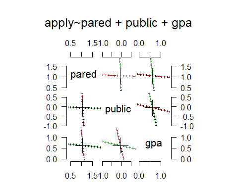
> m3 <- update(m, Hess=TRUE)> pr <- profile(m3)> confint(pr)
## 2.5 % 97.5 % ## pared 0.5281772 1.5721695 ## public -0.6522008 0.5191415 ## gpa 0.1076189 1.1309092
> plot(pr)
> pairs(pr)
Conclusion
In this article, I shared my understanding of using multinomial and ordinal regression in R. These techniques are used when the dependent variable has levels that are either ordered or unordered. I’d suggest you pay attention to the interpretation aspect of the model. Coding is relatively easy, but unless you know what’s resulting, your learning will be incomplete.
There are many essential factors such as AIC and residual values to determine the effectiveness of the model. If you still struggle to understand them, I’d suggest you brush your basics of logistic regression. This should help you in understanding this concept better.
Frequently Asked Questions
A. Multinomial logistic regression is used to model the relationship between a categorical dependent variable with more than two categories and one or more independent variables. It can be applied in a variety of fields such as predicting customer behavior, medical research, political science, and image classification. The goal is to predict the probability of each category of the dependent variable based on the values of the independent variables.
A. Logistic regression helps to model the relationship between a binary dependent variable and one or more independent variables. On the other hand, multinomial logistic regression helps in modeling the relationship between a categorical dependent variable with more than two categories and one or more independent variables. Logistic regression predicts the probability of one outcome, while multinomial logistic regression predicts the probability of multiple outcomes simultaneously.
A. Ordinal logistic regression is a statistical method used to analyze the relationship between an ordinal dependent variable and one or more independent variables. It helps to model outcomes such as satisfaction levels or grades. The goal is to predict the probability of an observation belonging to a certain category or a higher category, based on the values of the independent variables.


Thanks, with your code I can run the actual examples, I learnt much from your blog, please keep it up, regards
Hi Sray, Thanks for writing such a marvelous article, I thoroughly enjoyed reading each bit !!! I have one question which I believe is pertinent to OLR. I am trying to establish a relationship strength where my Y is Discrete and X is Continuous. In your opinion which analysis can help me to achieve this as standard correlation theories will not work in this scenario. Later I would like to create a model around it. Just so let you know Y is survey Results (5 Categories) and X is a sentiment score.
Comments are Closed