How to perform feature selection (i.e. pick important variables) using Boruta Package in R ?
Introduction
Variable selection is an important aspect of model building which every analyst must learn. After all, it helps in building predictive models free from correlated variables, biases and unwanted noise.
A lot of novice analysts assume that keeping all (or more) variables will result in the best model as you are not losing any information. Sadly, that is not true!
How many times has it happened that removing a variable from the model has increased your model accuracy ?
At least, it has happened to me. Such variables are often found to be correlated and hinder achieving higher model accuracy. Today, we’ll learn one of the ways of how to get rid of such variables in R. I must say, R has an incredible CRAN repository. Out of all packages, one such available package for variable selection is Boruta Package.
In this article, we’ll focus on understanding the theory and practical aspects of using Boruta Package. I’ve followed a step wise approach to help you understand better.
I’ve also drawn a comparison of boruta with other traditional feature selection algorithms. Using this, you can arrive at a more meaningful set of features which can pave the way for a robust prediction model. The terms “features”, “variables” and “attributes” have been used interchangeably, so don’t get confused!

What is Boruta algorithm and why such a strange name ?
Boruta is a feature selection algorithm. Precisely, it works as a wrapper algorithm around Random Forest. This package derive its name from a demon in Slavic mythology who dwelled in pine forests.
We know that feature selection is a crucial step in predictive modeling. This technique achieves supreme importance when a data set comprised of several variables is given for model building.
Boruta can be your algorithm of choice to deal with such data sets. Particularly when one is interested in understanding the mechanisms related to the variable of interest, rather than just building a black box predictive model with good prediction accuracy.
How does it work?
Below is the step wise working of boruta algorithm:
- Firstly, it adds randomness to the given data set by creating shuffled copies of all features (which are called shadow features).
- Then, it trains a random forest classifier on the extended data set and applies a feature importance measure (the default is Mean Decrease Accuracy) to evaluate the importance of each feature where higher means more important.
- At every iteration, it checks whether a real feature has a higher importance than the best of its shadow features (i.e. whether the feature has a higher Z score than the maximum Z score of its shadow features) and constantly removes features which are deemed highly unimportant.
- Finally, the algorithm stops either when all features gets confirmed or rejected or it reaches a specified limit of random forest runs.
What makes it different from traditional feature selection algorithms?
Boruta follows an all-relevant feature selection method where it captures all features which are in some circumstances relevant to the outcome variable. In contrast, most of the traditional feature selection algorithms follow a minimal optimal method where they rely on a small subset of features which yields a minimal error on a chosen classifier.
While fitting a random forest model on a data set, you can recursively get rid of features in each iteration which didn’t perform well in the process. This will eventually lead to a minimal optimal subset of features as the method minimizes the error of random forest model. This happens by selecting an over-pruned version of the input data set, which in turn, throws away some relevant features.
On the other hand, boruta find all features which are either strongly or weakly relevant to the decision variable. This makes it well suited for biomedical applications where one might be interested to determine which human genes (features) are connected in some way to a particular medical condition (target variable).
Boruta in Action in R (Practical)
Till here, we have understood the theoretical aspects of Boruta Package. But, that isn’t enough. The real challenge starts now. Let’s learn to implement this package in R.
First things first. Let’s install and call this package for use.
> install.packages("Boruta")
> library(Boruta)
Now, we’ll load the data set. For this tutorial I’ve taken the data set from Practice Problem Loan Prediction
> setwd("../Data/Loan_Prediction")
> traindata <- read.csv("train.csv", header = T, stringsAsFactors = F)
Let’s have a look at the data.
> str(traindata)
> names(traindata) <- gsub("_", "", names(traindata))
gsub() function is used to replace an expression with other one. In this case, I’ve replaced the underscore(_) with blank(“”).
Let’s check if this data set has missing values.
> summary(traindata)
We find that many variables have missing values. It’s important to treat missing values prior to implementing boruta package. Moreover, this data set also has blank values. Let’s clean this data set.
Now we’ll replace blank cells with NA. This will help me treat all NA’s at once.
> traindata[traindata == ""] <- NA
Here, I’m following the simplest method of missing value treatment i.e. list wise deletion. More sophisticated methods & packages of missing value imputation can be found here.
> traindata <- traindata[complete.cases(traindata),]
Let’s convert the categorical variables into factor data type.
> convert <- c(2:6, 11:13)
> traindata[,convert] <- data.frame(apply(traindata[convert], 2, as.factor))
Now is the time to implement and check the performance of boruta package. The syntax of boruta is almost similar to regression (lm) method.
> set.seed(123)
> boruta.train <- Boruta(LoanStatus~.-LoanID, data = traindata, doTrace = 2)
> print(boruta.train)
Boruta performed 99 iterations in 18.80749 secs.
5 attributes confirmed important: ApplicantIncome, CoapplicantIncome,
CreditHistory, LoanAmount, LoanAmountTerm.
4 attributes confirmed unimportant: Dependents, Education, Gender, SelfEmployed.
2 tentative attributes left: Married, PropertyArea.
Boruta gives a crystal clear call on the significance of variables in a data set. In this case, out of 11 attributes, 4 of them are rejected and 5 are confirmed. 2 attributes are designated as tentative. Tentative attributes have importance so close to their best shadow attributes that Boruta is not able to make a decision with the desired confidence in default number of random forest runs.
Now, we’ll plot the boruta variable importance chart.
By default, plot function in Boruta adds the attribute values to the x-axis horizontally where all the attribute values are not dispayed due to lack of space.
Here I’m adding the attributes to the x-axis vertically.
> plot(boruta.train, xlab = "", xaxt = "n")
> lz<-lapply(1:ncol(boruta.train$ImpHistory),function(i)

boruta.train$ImpHistory[is.finite(boruta.train$ImpHistory[,i]),i])
> names(lz) <- colnames(boruta.train$ImpHistory)
> Labels <- sort(sapply(lz,median))
> axis(side = 1,las=2,labels = names(Labels),

at = 1:ncol(boruta.train$ImpHistory), cex.axis = 0.7)
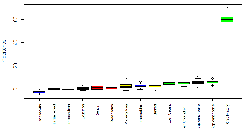
Blue boxplots correspond to minimal, average and maximum Z score of a shadow attribute. Red, yellow and green boxplots represent Z scores of rejected, tentative and confirmed attributes respectively.
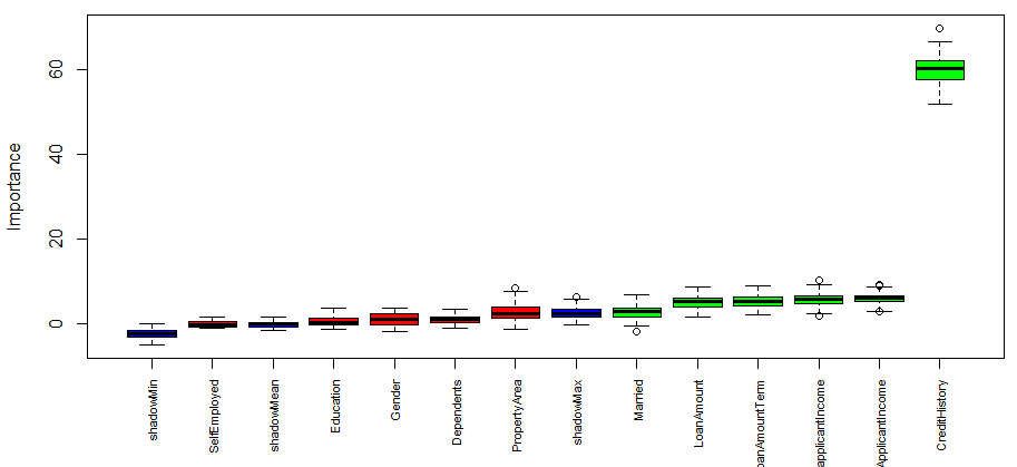
Now is the time to take decision on tentative attributes. The tentative attributes will be classified as confirmed or rejected by comparing the median Z score of the attributes with the median Z score of the best shadow attribute. Let’s do it.
> final.boruta <- TentativeRoughFix(boruta.train)
> print(final.boruta)
Boruta performed 99 iterations in 18.399 secs.
Tentatives roughfixed over the last 99 iterations.
6 attributes confirmed important: ApplicantIncome, CoapplicantIncome,
CreditHistory, LoanAmount, LoanAmountTerm and 1 more.
5 attributes confirmed unimportant: Dependents, Education, Gender, PropertyArea,
SelfEmployed.
Boruta result plot after the classification of tentative attributes
It’s time for results now. Let’s obtain the list of confirmed attributes
> getSelectedAttributes(final.boruta, withTentative = F)
[1] "Married" "ApplicantIncome" "CoapplicantIncome" "LoanAmount"
[5] "LoanAmountTerm" "CreditHistory"
We’ll create a data frame of the final result derived from Boruta.
> boruta.df <- attStats(final.boruta)
> class(boruta.df)
[1] "data.frame"
> print(boruta.df)
meanImp medianImp minImp maxImp normHits decision
Gender 1.04104738 0.9181620 -1.9472672 3.767040 0.01010101 Rejected
Married 2.76873080 2.7843600 -1.5971215 6.685000 0.56565657 Confirmed
Dependents 1.15900910 1.0383850 -0.7643617 3.399701 0.01010101 Rejected
Education 0.64114702 0.4747312 -1.0773928 3.745441 0.03030303 Rejected
SelfEmployed -0.02442418 -0.1511711 -0.9536783 1.495992 0.00000000 Rejected
ApplicantIncome 6.05487791 6.0311639 2.9801751 9.197305 0.94949495 Confirmed
CoapplicantIncome 5.76704389 5.7920332 1.9322989 10.184245 0.97979798 Confirmed
LoanAmount 5.19167613 5.3606935 1.7489061 8.855464 0.88888889 Confirmed
LoanAmountTerm 5.50553498 5.3938036 2.0361781 9.025020 0.90909091 Confirmed
CreditHistory 59.57931404 60.2352549 51.7297906 69.721650 1.00000000 Confirmed
PropertyArea 2.77155525 2.4715892 -1.2486696 8.719109 0.54545455 Rejected
Let’s understand the parameters used in Boruta as follows:
- maxRuns: maximal number of random forest runs. You can consider increasing this parameter if tentative attributes are left. Default is 100.
- doTrace: It refers to verbosity level. 0 means no tracing. 1 means reporting attribute decision as soon as it is cleared. 2 means all of 1 plus additionally reporting each iteration. Default is 0.
- holdHistory: The full history of importance runs is stored if set to TRUE (Default). Gives a plot of Classifier run vs. Importance when the plotImpHistory function is called.
For more complex parameters, please refer to the package documentation of Boruta.
Boruta vs Traditional Feature Selection Algorithm
Till here, we have learnt about the concept and steps to implement boruta package in R.
What if we used a traditional feature selection algorithm such as recursive feature elimination on the same data set. Do we end up with the same set of important features? Let us find out.
Now, we’ll learn the steps used to implement recursive feature elimination (RFE). In R, RFE algorithm can be implemented using caret package.
Let’s start by defining a control function to be used with RFE algorithm. We’ll load the required libraries:
> library(caret)
> library(randomForest)
> set.seed(123)
> control <- rfeControl(functions=rfFuncs, method="cv", number=10)
Here we have specified a random forest selection function through rfFuncs option (which is also the underlying algorithm in Boruta)
Let’s implement the RFE algorithm now.
> rfe.train <- rfe(traindata[,2:12], traindata[,13], sizes=1:12, rfeControl=control)
I’m sure this is self explanatory. traindata[,2:12] refers to selecting all independent variables except the ID variable. traindata[,13] selects only the dependent variable. It might take some time to run.
We can also check the outcome of this algorithm.
> rfe.train
Recursive feature selection
Outer resampling method: Cross-Validated (10 fold)
Resampling performance over subset size:
Variables Accuracy Kappa AccuracySD KappaSD Selected
1 0.8083 0.4702 0.03810 0.1157 *
2 0.8041 0.4612 0.03575 0.1099
3 0.8021 0.4569 0.04201 0.1240
4 0.7896 0.4378 0.03991 0.1249
5 0.7978 0.4577 0.04557 0.1348
6 0.7957 0.4471 0.04422 0.1315
7 0.8061 0.4754 0.04230 0.1297
8 0.8083 0.4767 0.04055 0.1203
9 0.7897 0.4362 0.05044 0.1464
10 0.7918 0.4453 0.05549 0.1564
11 0.8041 0.4751 0.04419 0.1336
The top 1 variables (out of 1):
CreditHistory
This algorithm gives highest weightage to Credit History. Now, we’ll plot the result of RFE algorithm and obtain a variable importance chart.
> plot(rfe.train, type=c("g", "o"), cex = 1.0, col = 1:11)
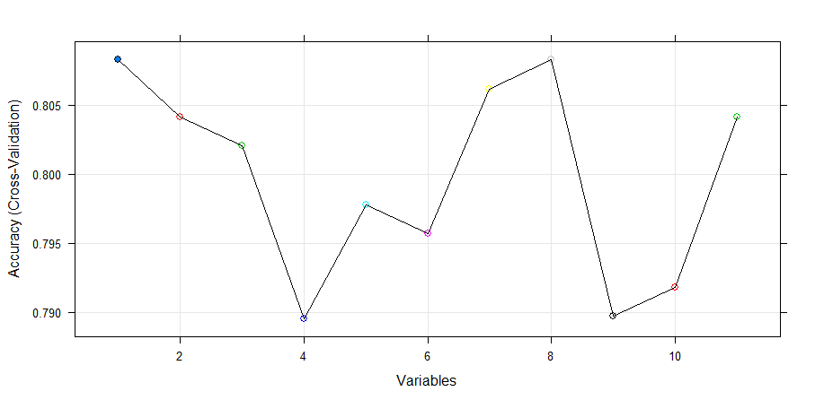
Let’s extract the chosen features. I am confident it would result in Credit History.
> predictors(rfe.train)
[1] "CreditHistory"
Hence, we see that recursive feature elimination algorithm has selected “CreditHistory” as the only important feature among the 11 features in the dataset.
As compared to this traditional feature selection algorithm, boruta returned a much better result of variable importance which was easy to interpret as well ! I find it awesome to work on R where one has access to so many amazing packages. I’m sure there would be many other packages for feature selection. I’d love to read about them.
End notes
Boruta is an easy to use package as there aren’t many parameters to tune / remember. You shouldn’t use a data set with missing values to check important variables using Boruta. It’ll blatantly throw errors. You can use this algorithm on any classification / regression problem in hand to come up with a subset of meaningful features.
In this article, I’ve used a quick method to impute missing value because the scope of this article was to understand boruta (theory & practical). I’d suggest you to use advanced methods of missing value imputation. After all, information available in data is all we look for ! Keep going.
Did you like reading this article ? What other methods of variable selection do you use? Do share your suggestions / opinions in the comments section below.
About the Author
 Debarati Dutta is MA Econometrics graduate from University of Madras. She has more than 3 years of experience in data analytics and predictive modeling across multiple domains. She has worked in companies such as Amazon, Antuit, Netlink. Currently, she’s based out of Montreal, Canada.
Debarati is the first winner of Blogathon. She won amazon voucher worth INR 5000.


Gr8 Share Debrati. I was looking for the same kind of info. Keep sharing. Thanks.
Thanks Sreenivas. Glad that it helped.
Beautiful, meaningful info, thanks a lot
Thank you so much Dr. Samuel.
Hi, This is not the best package for the determination of the importance of predictors. See this article.https://www.mql5.com/en/articles/2029
Hi Vlad, Thanks for the interesting article. Well, I would say "best" is more likely a relative term which depends a lot on the problem we have in hand as well as our needs. As mentioned in another comment, if prediction accuracy is your only concern, it might / might not be the best method for feature selection. But, if you are also interested in understanding the relationships in your data, it would do a much better job. Hence, application of machine learning techniques involve a lot of trial and error to arrive at the "best" method.
Great tutorial! Thanks!
Thanks @geneseo2000.
Hi Debrati, Has this model of feature selection helped in improving the predictions.
Hi Mathew, Good question. Well, the answer wouldn't be yes in all cases. In case you only care about good prediction accuracy, it might / might not be the best method for feature selection. But, if you are also interested in inference, it will help you come up with a subset of features, both strongly and weakly relevant to the outcome variable. In this case, although the feature sets obtained from the two methods are quite different, but still it would have very negligible difference in prediction accuracy. It is due to the fact that the extra variables confirmed by Boruta are weakly relevant to the outcome variable (as evident from the Boruta plot) and hence, might not be playing a major role in prediction accuracy. This might differ from case to case. Hope this helps.
Really useful package and thanks Debarati really helpful article . only one Comment for the readers please do change Loan_status to LoandStatus and Loan_ID to LoanID , otherwise it will throw an error
Hi Hunaidkhan, Glad that it helped. And thank you so much for pointing it out. Cleaning the variable names using gsub is an optional step and can be avoided.
thanks for this info , please can you send me the traindata thanks
Hi @joo, Glad that you liked it. Can you please send me your e-mail ID?
It would be nice to obtain a decent print of this and other articles.
Hi Michael, Glad that you liked it.
Hi, Nice article! This seems to be computationally very expensive. I have a dataset which has 80K rows and 150 columns and Boruta feature selection is taking over 3 hours... Is there any way to optimize the calculations?
Hi Pallavi, Glad that it helped. Well, it is computationally expensive as it is a permutation-based feature selection method. You can try out a couple of things to make it a little faster. Try specifying holdHistory = F while implementing boruta to prevent it from saving the full history of variable importance runs. boruta.train <- Boruta(Loan_Status~.-Loan_ID, data = traindata, doTrace = 2, holdHistory = F) Altenatively, you can also try decreasing the value of maxRuns parameter in case you are not getting any tentative attributes with the default number of random forest runs. By default, Boruta uses Random forest mean decrease accuracy as the variable importance measure. You can try using a faster Random ferns based variable importance measure. Random ferns is a simplified variation of random forest algorithm. install.packages("rFerns") library(rFerns) set.seed(123) boruta.train <- Boruta(LoanStatus~.-LoanID, data=traindata, doTrace = 2, getImp=getImpFerns, holdHistory = F) In this case, you might obtain a different subset of features as the underlying algorithm is different. Hope this helps.
Really nice article thanks. Donyou know if the algorithm can be implemented in Python?
Hi Michael, Glad that you liked it. The Python implementation of Boruta can be found in this github account. https://github.com/danielhomola/boruta_py
I've DATE data in my csv file. Boruta can diffentiate them, but RFE cannot take in DATE format ? it seems RFE can take in only numerical variables ? Eg mydate is "3/10/2016"
Hi james, I presume your mydate variable is of class "character" until you convert it to R date format. Well, boruta can handle predictor variables from classes numeric, factor and character but RFE is only able to handle variables of classes numeric and factor. The reason behind this is although both the algorithms function as wrappers around random forest, they implement random forest algorithm using two different R packages. Boruta runs random forest from ranger package which allows automatic coercion of character variables to factor labels whereas RFE runs the algorithm from randomForest package which doesn't automatically convert the character variables to factors labels. So, in case of RFE, the character variables in the input dataset are coerced to numeric and hence, NAs will be introduced by coercion. Hope this helps.
Good one
thanks for sharing this nice information.wonderful explanation.your way of explanation is good.,it was more impressive to read ,which helps to design more in effective ways
Really good article. when I tried the same approach on my data, I received a bit different result. I found 4 variables through Boruta and 5 through the variables, even the 4 variables are not subset of the 5 variables. I am wondering what could be the reason of this.
Thanks Debarati for sharing this. Though I have not tested this, but have few questions: 1. If my ultimate aim is to use a GLM (Generalized Linear Model), do you think it's useful to use a random forest based feature analysis, or should I try something else which are based on GLM methods? 2. What's the 'importance' criterion in this model based on (e.g. Goodness of fit, information criterion,...) 3. Do you think it's useful for regression analysis where the predicted value is a continuous variable?
Have you tried Gradient Boosting based Feature Importance? It's a very powerful technique. It gave superior results to Random Forest results on all my datasets
Hi, Thanks for sharing the information. Although you explained it clearly the logic behind the Boruta package, I still surprised that most of the features shown as confirmed are not significant in simple glm. Here my analysis is not to improve the accuracy of the model but towards understanding the relationships within the data. I also tried with simple t-test/chi square on the confirmed features and found all numeric features are not significant. As you pointed Boruta is a wrapper algorithm around random forest and looks like it is biased towards numeric features. My analysis suggests cforest from party package is providing reasonable features which are aligned with my EDA like t-test/chi square test .Even for finding strong relationship with target variable, not sure this package is doing justice to it.
Great Share
Hello #Debarathi Dutta , This really helped to improve my model. Thank you very much for sharing .
Thank you for the article. Appreciate it What benefit this package adds on top of Random Forest if I were to directly use Random Forest? Thank you for your help
Good information! But I have a question. In result of Boruta, what is the normHits? Can you explain formulation??? In Boruta PDF, only explain what is the normHits shortly. But I want to know formulation.
Hello Debrati, Thank you for sharing such a informative post. I have couple of questions: How good is this in dealing with outilers? Should we treat them before applying Boruta? For categorical variables, should we create dummy variables and run Boruta or before creating any dummy variables should we run? Thanks,
Good article. Wanted to run this code and play around, but could not find the data set for download. Could you share the data set in anyway?
Hi everybody, I was trying to download the dataset used in this tutorial but I couldn't find it. Could someone help me, please? On another hand, I don´t know if it is right to ask you by this way, but I was working on a dataset which has many features related each other, it is a data set of cutting tools machines, I aim to get a model to predict some cutting parameters, thus I was trying to apply something to analyze the importance of each feature, not only to reduce them, also to understand their impact to my results. I am quite sure if random forest or Boruta could they help me because I m not looking for a tree decision. Could someone give an advice about this? Thank so much
This appears to be just what I need. Thanks so much. Any updates or other packages that may have come over the past year? Thanks again, Stephen
Hello, Great articles. Thanks for sharing!
Can't find the dataset in the link provided. Can you please share the dataset so that I can do this hands on ?
How do you compare this with the one done by RandomForest? Thank you
Great write up Debarthi... Found the article very informative and lucid explanation. Though I have one question.. I am working on problem set having 2489 attributes. I am planning to use nnets to predict the output variable. If I have to apply Boruta on the dataset ( for which underlying algo is random forest) , how will the model behave. Though i will be trying it out , but wanted to know if you can throw some light on it . Any help is appreciated. Thanks
Great write up Debarthi... Found the article very informative and lucid explanation. Though I have one question.. I am working on problem set having 2489 attributes. I am planning to use nnets to predict the output variable. If I have to apply Boruta on the dataset ( for which underlying algo is random forest) , how will the model behave. Though i will be trying it out , but wanted to know if you can throw some light on it . Your help is appreciated. Thanks
Can anyone please describe what the upper and lower bar correspond for in that plot? And also what is the bold line within each box?
I used both Boruta and rfe feature selection method on the kaggle titanic dataset. To my surprise Boruta declared all the predictors as important while rfe picked up only 4 out of 8 variables. I built a rf model using both suggestions and the rfe method gave me a better model compared to boruta. Is there any reason for such behaviour ?
Thank you for this great explanation of two different feature selection algorithms. However, just because RFE selected only 1 feature out of 11 while boruta selected 6 features, doesn't mean that boruta is superior. I wished you developed two different models using both RFE's and boruta's features then compared their accuracy or another metric in order to see which is better. Best regards,
Dear Debarati; Great article, really helpful but the data link isn't working anymore, can you please upload another link, again thank you Debarati
Can somebody send the training data for this problem!
Hi Ashay, You can download the dataset from this link.
Wow, great wrap up. Probably all the needed to jump start knowledge in the one place and served in a comprehensive way. Many thanks!