Tutorial – Data Science at Command Line with R & Python (Scikit Learn)
Introduction
The thought of doing Data Science at Command Line may possibly cause you to wonder, what new devilry is that?
As if, it weren’t enough that, an aspiring data scientist has to keep up with learning, Python / R / Spark / Scala / Julia and what not just to stay abreast, that someone’s adding one more to that stack?
Worry not, it’s not something new (a part of it is new though) but something that’s already existed for a while and with a bit of fresh perspective might just become a quintessential part of your data-science-workflow.
My inspiration to write this article derived from a book Data science at the command line by Jeroen Janssens. Since then, I’ve been reading up and applying things I learnt by using it in my workflow.
I hope, by demonstrating some quick hands-on examples in this article, I can whet your appetite for more command line goodness and hopefully you’ll get brand new skill-set in your arsenal. I’ve explained every bit of code to help you understand command line faster.
Note: For modeling purpose, I’ve used linear regression, random forest and gradient boosting algorithm.

Table of Contents
- Why Data Science at Command Line?
- Data Science is OSEMN
- Required Installations
- Part 1 : Obtain | Scrub | Explore Data
- Practice Problem – Black Friday
- Part 2 : Visualize – Using R on Command Line
- Part 3 : Model with Scikit-Learn on Command Line
- Summary
- End Notes:
- General
- About AWK & SED
Why Data Science @ the Command Line?
Given that data science is such a multi-disciplinary field, we have folks from wide variety of professional background and skills; one of the most common ones being some experience using the Unix command line, even if it be for basic actions like cp / grep / cat / wc / head / tail / awk */ sed* / bash*.
The command line has existed for a long time and can be found on any Unix based OS. Even, Microsoft Windows has now come out with a bash shell. So, it becomes pretty appealing to have one system to carry out Data Science tasks.
Taking the ideas from the UNIX philosophy, of text being the input /output most command produce and that a UNIX command performing one type of action and doing it well; piping these commands together, we can augment these in our data science workflows.
UNIX pipes allow us to pass on the output of one command as input for the next one. Have a look at the GNU site to see the various free and robust tools developed by the OS community – quite interesting to have a wide-array of tools at your disposal to carry out tasks. Lastly, command line tasks can be automated and operated in parallel thereby making it quick and efficient.
In the age of Big Data and IoT, the appeal for command line tools still persists. Imagine, instead of moving around large amounts of data, you could analyse it, visualise it, and get a feel for it directly from the command line!
Does it mean, that we should do away with R / Python or others and do everything on the command line? Perhaps not, rather just use the right tool at the right time in the right context and use the command line to supplement R / Python / other tools.
A popular taxonomy of data science describes it as OSEMN (pronounced: Awesome)
(Dragon due of GoT Finale still fresh in my mind)
- O: Obtain, data from various sources
- S: Scrub, perform data wrangling
- E: Explore
- M: Model
- N: Interpret
In practice, OSEMN tends to be a cyclical process as opposed to a purely linear one. In this article, we shall only be covering the OSEM parts of the OSEMN acronym.
Required Installations
Before we can get started, let’s ensure we have everything required to work on command line:
Packages & Commands
- All: The easiest way to get along doing hands on exercises is to use the virtual machine (VM) created by Jeroen Janssen (here) with all tools pre-installed. Also, you can find the code on Jeroen’s git here or buy the book (I don’t get anything out of this).
- Linux & OSX: If you are confident about command line, most packages can be easily installed on Linux / Mac based machines using
pip installorapt-getorbrew(Mac OSX). Some of them require special package managers likenpmto be installed and some (such asawk,sed,cat,head,tail,grep,nletc.) are already pre-installed on Linux / Mac machines. It should essentially be a one-time installation. I personally prefer to install them once and be done with it. Jeroen’s book list all the commands used in the appendix and ways to install them in bit more detail than what I have.
To carry out the exercises, you’ll mostly need datamash, csvkit, and skll — which can be installed as follows,
pip install datamash- Datamash Documentation here.
pip install csvkit- CSVKIT Documentation here.
- Rio & Header are available on Jeroen’s Git here. You’ll need to extend your Unix PATH so the bash shell knows where to look for the command. Here is how you can extend your Unix PATH.
pip install skll- If using python 2.7,
pip install configparser futures logutils
Not the most important right away,
pip install cowsay(for the dragon-image)pip install imagemagickORbrew install imagemagick(mac only)
Windows: You’ll need the same packages as in Linux / OSX section. It’s just you might have to put more effort to install it.
- Windows 10 now comes with the functionality to install a bash shell. Below are the links to Microsoft’s website, explaining how to use bash shell. I haven’t used it personally, so can’t comment on how straightforward it is to install packages there.
- For other Windows versions: use Cygwin and try to install the packages.
- As a last resort, you can use the “Free Tier” from Amazon AWS. More info here. Just pick up any Linux instance Ubuntu or Open Suse, install the same packages as above and get going.
Once you’ve installed the tools, and need help, you can use the Unix command man command-name or command-name --help on the command line to get further help or our good friend Google is always there!
Part 1: Obtain | Scrub | Explore Data
We’ll use the data set from Black Friday Practice Problem. Feel free to work together on your command line as we go through the examples – just make sure, you have installed all the packages and refer to end notes if you get stuck.
After you’ve downloaded the file from link above, unzip it in a folder and rename the extracted csv file as bfTrain.csv. Ensure that you change your present working directory to the folder where you’ve downloaded & extracted the csv file.
Use the “cd” command to change directory
Let’s look at some of the most common tasks to be performed with a new data set. We’ll now check out the dimension of this data set using 2 methods (you can use any):
> cat bfTrain.csv | awk -F, ' END {print " #Rows = " NR, " # Columns = " NF}’

Output: #Rows = 550069  # Columns = 12 #Method 1
> cat bfTrain.csv | datamash –t, check
Output: 550069 lines, 12 fields #Method 2
We know the file is comma separated and the first row is a header. In method 1, AWK is used to count the #Rows and #Columns and display it in a nice format. Just for fun, prefix the command, time to both the methods above to compare the 2 methods, like this:
> time cat bfTrain.csv | datamash –t, check
Let’s perform basic steps of data exploration now:
1. Columns: Now, we’ll check for available columns in the data set:
> head –n 1 bfTrain.csv | tr ‘,’ ‘\n’ | nl

Output
1 User_ID
2 Product_ID
3 Gender
4 Age
5 Occupation
6 City_Category
7 Stay_In_Current_City_Years
8 Marital_Status
9 Product_Category_1
10 Product_Category_2
11 Product_Category_3
12 Purchase
In the command above, we just took the first row of the file and used tr to transform the commas (remember, it’s a csv file) to a new-line separator. nl is used to print line numbers.
2. Rows: Check first few rows of the data
> head –n 5 bfTrain.csv | csvlook
In this command, we used the regular head command to select top 5 rows and pipe it to command csvlook to present it in a nice tabular format.
In case you’re having difficulty viewing the output on your command line, try the following to view a section of the data at a time. Let’s display first 5 columns of the file:
> head bfTrain.csv | csvcut –c 1-5 | csvlook
Now, displaying the remaining columns:
> head bfTrain.csv | csvcut –c 6- | csvlook
3. Value counts: Let’s dive deeper into the variables. Let’s see how many male / female respondents exist in the data.
> cat bfTrain.csv | datamash -t, -s -H -g 3 count 3 | csvlook
The cat command just pips in the file. Then, using datamash, we ask to group by the 3rd column (Gender) and do a count on the same. The datamash documentation explains all the various options used.
Tip: In case your data has too many columns, it might be a good idea to use csvcut to just select the columns you need and use it for further processing.
Exercise: Try answering the following questions:-
- How many people live in the different cities?
- Can you find all the unique Occupations? (Hint: use command ‘unique’)
4. groupBy Stats: Is there a difference in the purchase amount by gender?
There are many ways to answer this. We can use something everyone would be very familiar with i.e. SQL – yes we can write sql queries directly on the command line to query a csv file.
> cat bfTrain.csv | csvsql --query "select Gender,avg(Purchase), min(Purchase), max(Purchase) from stdin group by 1" | csvlook
5. crosstabs: How are men / women distributed by age group?
> cat bfTrain.csv | datamash -t, -s -H crosstab 4,3 | csvlook
6. scrub data: Just for argument’s sake, assume that we have to remove the ‘+’ sign from the observations of “age” column. We can do it as follows:
> cat bfTrain.csv | sed ‘s/+//g’ > newFile.csv
Here, we use SED to remove the ‘+’ sign in the Age column.
7. NA / nulls: How do we find out if the data contains NAs?
> csvstat bfTrain.csv --nulls
Here, we call upon csvstat and pass the argument --nulls to get a True/False style output per column.
Exercise: Pass the following arguments one-at-a-time to csvstat to get other useful info about the data –min, –max , –median, –unique
Hopefully by now, you might have realized that command line can be pretty handy and fast while working on a data set. However, until here we’ve just scratched the surface by doing exploratory work so far. To drive the point home, just reflect on the point that we did all of the things above, without actually loading the data (in memory as in R or Python). Pretty cool eh?
8. Different Data Formats
Perhaps you’ve noticed that until now, we’ve only used data in nicely formatted csv or txt files. But, surely in the age of Big Data and IoT that’s not all what command line can handle, can it? Let’s look at some available options:
1. in2csv
It’s part of the csvkit command line utility. It’s a really awesome command line tool that can handle csv, geojson, json, ndjson, xls, xlsx, and DBase DBF.
2. Convert xlsx to csv
> curl -L -O https://github.com/onyxfish/csvkit/raw/master/examples/realdata/ne_1033_data.xlsx > ne_1033_data.xlsx
> in2csv ne_1033_data.xlsx > ne_1033_data.csv
In here, we’ve simply used curl to download the excel file and save it. Then, we used in2csv to convert excel to a csv file of same name.
3. Json to csv
Utility tools such as in2csv and jq allow us to handle json and other data formats.
4. Databases
Again csvkit comes to the rescue here, providing a tool sql2csv that allows us to query on several different databases (e.g. Oracle, MySQL, and Postgres etc.).
Part 2: Visualize – Using R on the Command Line
How cool would it be if we could leverage our R knowledge, scripts directly on the command line?
As you might have guessed by now, there exists a solution for this too. Jeroen (the author of Data Science at Command Line) has created many handy tools, and one of them is Rio. It’s an acronym for R input/ output. Rio is essentially a wrapper function around R that allows us to use R commands on the command line.
Let’s get cracking!
#Summary Stats
> cat bfTrain.csv | Rio –e ‘summary(df$Purchase)’
#calculating correlation between age and purchase amount
> cat bfTrain.csv | csvcut –c Age,Purchase | cut –d ‘-‘ –f 2 | sed ‘s/+//g’ | Rio –f cor | csvlook
Let’s understand how it works. Here, we select the columns Age, Purchase using csvcut. Since, Age is presented as a range of values like 0-17, 26-35 etc., we use cut to select the upper limit of the age range (think of it as using substring to select a specific portion of a text).
Next, we remove the ‘+’ sign from the Age column using sed. Finally, we make a call to Rio to check correlation between the 2 columns and present it nicely using csvlook.
Data Visualisation: Let’s use another data set now. We’ll refer to the UCI Irvine website and download “Abalone” dataset. This data set is about predicting the age of abalone (oyster like sea-creature) from physical measurements. The target column in the data is Rings.
#Getting Actual Data
> curl http://archive.ics.uci.edu/ml/machine-learning-databases/abalone/abalone.data > abalone.csv
#Getting Data Description
> curl http://archive.ics.uci.edu/ml/machine-learning-databases/abalone/abalone.names > abaloneNames.txt
#View sample data
> head abalone.csv | csvlook
#Create a scatterplot
> cat abalone.csv | csvcut –c Rings,Diameter,Sex | Rio –ge ‘g+geom_point(aes(Diameter,Rings,color=factor(Sex)))’ | display
Let’s understand how the above code works!
As usual, we take the input data file, select the columns we need. Then, we call Rio and the R-code to create a scatter plot colour coded by Sex (M / F) and save it to a file. The code to create R-graphs is that of ggplot2.
If you are unable to see the image , just change the command above as:
> cat abalone.csv | csvcut –c Rings,Diameter,Sex | Rio –ge ‘g+geom_point(aes(Diameter,Rings,color=factor(Sex)))’ > abaScatter.jpeg
This will redirect the output graph as a jpeg file into your current working directory. This is how it would look like: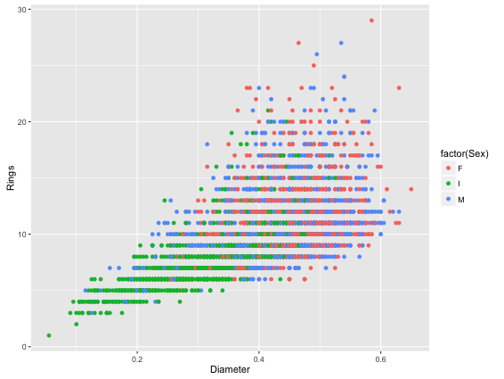
#Boxplot
> cat abalone.csv | csvcut –c Rings,Sex | Rio –ge ‘g+geom_boxplot(aes(Sex, Rings))’ > abaBoxP.jpeg
We used ggplot to produce a boxplot and divert it as a jpeg file in your current working directory.
Part 3: Modeling with Scikit-Learn on the Command Line
Now we come to the final and perhaps the most interesting part of modeling data on the command line with Scikit-learn. Let’s continue with the abalone data set used above.
We can extract the column names from the abaloneNames.txt file as:
> tail –n +89 abaloneNames.txt | awk ‘NR<10{print $1}’ | tr ‘\n’ ‘,’ | sed ‘s/,//9’
Output: Sex,Length,Diameter,Height,Whole,Shucked,Viscera,Shell,Rings
Let’s see what we just did.
- Here, I filtered the description file. Then, I used
awkto select 9 rows and printed them on the same line separated by commas usingtr. Later, I viewed theabaloneNames.txtfile in a text editor (for e.g. notepad++) to get the line #89. - Of course, we could have just copied the column names from the text file directly but I just wanted to show how we could do it automatically on the command line. We do this because in this case, data file doesn’t have headers.
We need to do some groundwork before we can start modelling. The steps are as follows,
- Add the column names to the data file.
- Add an id column (for e.g. 1,2,3…) at the start of the data file to easily identify the predictions later.
- Create a config file to set the parameters for the model.
Let’s do it.
1. Add the column names to the data file.
Now, we’ll extract the column names from the abaloneNames.txt and store it in a separate file abaloneCN.txt
> tail –n +89 abaloneNames.txt | awk ‘NR<10{print $1}’ | tr ‘\n’ ‘,’ | sed ‘s/,//9’ > abaloneCN.txt
> cat abalone.csv | header –e “cat abaloneCN.txt” > abalone_2.csv
In the command above, I used sed to remove the 9th comma. Then, I piped in the abalone.csv file and called upon the command header which is allowed us to header to a standard output / file. The abaloneCN.txt is then passed on to it and the output is directed to a new file called abalone_2.csv.
2. Add an id column at the start of the features.csv file
> mkdir train | cat abalone_2.csv | nl –s, -w1 –v0 | sed ‘1s/0,/id,’ > ./train/features.csv
Let’s see what we did:
- We created a new directory called folder, piped in the
abalone_2.csvfile, invoked thenlcommand as we used earlier to add numbers starting count at 0 and separated by a comma. - Finally, we called upon
sedto only replace0in the header row withid, and save the file asfeatures.csvunder the train directory.
3. Creating a config file
We’ll now create a config file which contains the model configurations. You can create it using any text editor; just remember to save it as “predict-rings.cfg”. It’s contents should be:
[General]
experiment_name = Abalone
task = cross_validate
[Input]
train_location = train
featuresets = [["features.csv"]]
learners = ["LinearRegression","GradientBoostingRegressor","RandomForestRegressor"]
label_col = Rings
[Tuning]
grid_search = false
feature_scaling = both
objective = r2
[Output]
log = output
results = output
predictions = output
Let’s understand it as well. Here we call the experiment, Abalone. We used 10-fold cross-validation and 3 modeling techniques (Linear Regression, Gradient Boosting, Random Forest). The target column is specified under, label_col as Rings. More Info about creating cfg files for run_experiment can be found here.
Now that the groundwork is done, we can call start modeling.
> run_experiment –l predict-rings.cfg
In this command, we call upon the run_experiment command to run the config file and start modeling. Be patient, this command might take time to run.
Once modeling is done, the results can be found under the “output” directory (created in the directory folder, where the command run_experiment was run from).
There are 4 types of files produced per modeling technique (for the 3 techniques we used here, we end up with 12 files). Files being (.log, .results, .results.json, .predictions) and a summary file (with suffix _summary) containing information about each fold. We can get the model summary as follows:
> cat ./output/Abalone_summary.tsv | csvsql –query “select learner_name, pearson FROM stdin WHERE fold = 'average' ORDER BY pearson DESC" | csvlook”
| learner_name | Pearson |
| RandomForestRegressor | 0.744 |
| GradientBoostingRegressor | 0.734 |
| LinearRegressor | 0.726 |
Let’s understand it now:
- First, we call upon
Abalone_summary.tsvfile. Using sql, we generated a summary of results. We see that random forest gives the best result in this case. The pearson score indicates the correlation between the true ranking (of the rings) and the predicted values. - We didn’t perform any feature engineering as this was just an exercise to show how we can model from the command line from the Scikit learn.
End Notes
General
- In case you find yourself using a set of commands in your workflow quite regularly, you can put them together in a bash script and reuse them time and again!
- It’s even possible to call bash command from IPython. Here’s an article describing it in detail.
About AWK / SED
- Perhaps may or may not have heard / used them before. This blog wasn’t meant as a class towards AWK & SED programming but just as a key point, remember,
- Awk excels are line and column level processing of files, whereas,
- SED (Stream Editor) excels at character level manipulation. SED commands tend to follow the general structure,
sed’s/old/new where old is what you want to replace and new is what you will replace it with. Essentially old and new are regular expressions.
This brings us to the end of this article. We’ve covered quite some ground – going through the already familiar data science tasks (getting data directly from the source, summarizing it, understanding it, plotting it, finally modeling it) and using a different way to approach them.
I hope you enjoyed working on data at command line (probably for the first time) and feel encouraged to explore it further. It can seem a bit daunting at first to remember the various options, tool names but it’s only a matter of little practice. In the world of fancy GUIs, a classical command line does still hold a certain allure for me.
My personal goal is to get proficient using command line tools more as part of my workflow and combine it with Vowpal Wabbit (read more here), which is an open source fast out-of-core learning system library and program.
About Author
Sandeep Karkhanis (@sskarkhanis) is passionate about numbers. He has worked in few industries mainly Insurance, Banking and Telcos. He is currently working as a Data Scientist in London. He strives to learn new ways of doing things. His primary goal is to use his data science skills for social causes and make human lives better. You can connect with Sandeep at [email protected]


