Essentials of Deep Learning: Getting to know CapsuleNets (with Python codes)

Introduction

Neural networks have been around since the last century but in the last decade, they have reshaped how we see the world. From classifying images of animals to extracting parts of speech, researchers are building deep neural networks in diverse and vast fields to push and break boundaries.

But as advancements in deep learning reach new heights, a new concept has lately been introduced that is a twist on the old neural network architecture – Capsule Networks. It improves on the effectiveness of the old traditional methods and understands even when presented with a situation that is shown from a different angle.

In this article, we will see why Capsule Networks are suddenly getting so much attention in the deep learning community, what the intuition behind this concept is and we will then do a code walk through to strengthen and solidify our concepts.

So are you ready? Let’s go!

Note: I suggest you go through the below articles before reading further in case you need to brush up your neural network concepts:

• Fundamentals of Deep Learning – Starting with Artificial Neural Network
• Tutorial on Optimizing Neural Networks using Keras
• Architecture of Convolutional Neural Networks (CNNs) Demystified

Table of Contents

1. Why is CapsuleNet getting so much attention?
2. Intuition behind Capsule Networks
3. Code Walkthrough of CapsNet on MNIST

Why is CapsuleNet getting so much attention?

You must have already heard the tales of CapsuleNets – but let us see it through with our eyes. To compare the power of this new architecture – let us monitor CapsNet on Analytics Vidhya’s Identify the Digits Problem.

Note – The code for this section is included in the “Code Walkthrough section”. Alternatively, you can check out the code on GitHub.

For the uninitiated, the Identify the Digits problem, as the name suggests, is simply a digit recognition problem. When given a simple black and white image, the user has to predict the number shown in it.

As this is an unstructured data problem, specific to image recognition, it is common knowledge that you should apply Deep Learning algorithms to get the best performance on the data. We will survey three Deep Learning architectures for this problem to check their performance, namely:

1. A simple Multi-layer Perceptron
2. Convolutional Neural Network
3. Capsule Network

Multi-layer Perceptron

For our first attempt, let us build a very simple Multi-layer Perceptron (MLP) for our problem. Below is the code to build an MLP model in keras:

# define variables
input_num_units = 784
hidden_num_units = 50
output_num_units = 10

epochs = 15
batch_size = 128

# create model
model = Sequential([
 Dense(units=hidden_num_units, input_dim=input_num_units, activation='relu'),
 Dense(units=output_num_units, input_dim=hidden_num_units, activation='softmax'),
])

# compile the model with necessary attributes
model.compile(loss='categorical_crossentropy', optimizer='adam', metrics=['accuracy'])

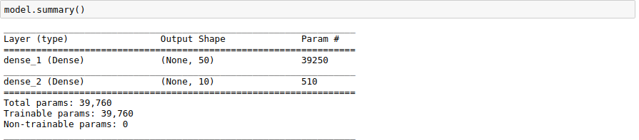
Below is our model summary:

Now after training for 15 epochs, here is the result we get:

Epoch 14/15
34300/34300 [==============================] - 1s 41us/step - loss: 0.0597 - acc: 0.9834 - val_loss: 0.1227 - val_acc: 0.9635
Epoch 15/15
34300/34300 [==============================] - 1s 41us/step - loss: 0.0553 - acc: 0.9842 - val_loss: 0.1245 - val_acc: 0.9637

Looks impressive for such a simple model!

Convolutional Neural Network (CNN)

Now we’ll move on to a more complex architecture, aka, Convolutional Neural Network (CNN). We have defined the model in the code below.

# define variables
input_shape = (28, 28, 1)

hidden_num_units = 50
output_num_units = 10

batch_size = 128

model = Sequential([
 InputLayer(input_shape=input_reshape),

Convolution2D(25, 5, 5, activation='relu'),
 MaxPooling2D(pool_size=pool_size),

Convolution2D(25, 5, 5, activation='relu'),
 MaxPooling2D(pool_size=pool_size),

Convolution2D(25, 4, 4, activation='relu'),

Flatten(),

Dense(output_dim=hidden_num_units, activation='relu'),

Dense(output_dim=output_num_units, input_dim=hidden_num_units, activation='softmax'),
])

model.compile(loss='categorical_crossentropy', optimizer='adam', metrics=['accuracy'])

Let’s print our model summary:

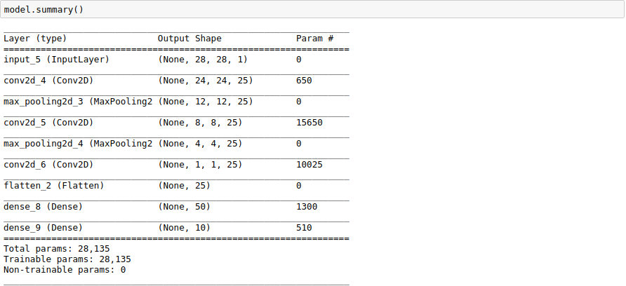
We see that our CNN model is deeper and more complex than our initial MLP model. Let’s see if that horsepower is appropriate.

Epoch 14/15
34/34 [==============================] - 4s 108ms/step - loss: 0.1278 - acc: 0.9604 - val_loss: 0.0820 - val_acc: 0.9757
Epoch 15/15
34/34 [==============================] - 4s 110ms/step - loss: 0.1256 - acc: 0.9626 - val_loss: 0.0827 - val_acc: 0.9746

We see that it takes more time to train our model. But its worth the effort as it gives a significant performance boost.

Capsule Network

Now let us check out the last architecture, the Capsule Network. As you might have guessed – it is bigger and even more complex than CNN. Below is the code to build it.

def CapsNet(input_shape, n_class, routings):
   x = layers.Input(shape=input_shape)

   # Layer 1: Just a conventional Conv2D layer
   conv1 = layers.Conv2D(filters=256, kernel_size=9, strides=1, padding='valid', activation='relu', name='conv1')(x)

   # Layer 2: Conv2D layer with `squash` activation, then reshape to [None, num_capsule, dim_capsule]
   primarycaps = PrimaryCap(conv1, dim_capsule=8, n_channels=32, kernel_size=9, strides=2, padding='valid')

   # Layer 3: Capsule layer. Routing algorithm works here.
   digitcaps = CapsuleLayer(num_capsule=n_class, dim_capsule=16, routings=routings,
   name='digitcaps')(primarycaps)

   # Layer 4: This is an auxiliary layer to replace each capsule with its length. Just to match the true label's shape.
   # If using tensorflow, this will not be necessary. :)
   out_caps = Length(name='capsnet')(digitcaps)

   # Decoder network.
   y = layers.Input(shape=(n_class,))
   masked_by_y = Mask()([digitcaps, y]) # The true label is used to mask the output of capsule layer. For training
   masked = Mask()(digitcaps) # Mask using the capsule with maximal length. For prediction

   # Shared Decoder model in training and prediction
   decoder = models.Sequential(name='decoder')
   decoder.add(layers.Dense(512, activation='relu', input_dim=16*n_class))
   decoder.add(layers.Dense(1024, activation='relu'))
   decoder.add(layers.Dense(np.prod(input_shape), activation='sigmoid'))
   decoder.add(layers.Reshape(target_shape=input_shape, name='out_recon'))

   # Models for training and evaluation (prediction)
   train_model = models.Model([x, y], [out_caps, decoder(masked_by_y)])
   eval_model = models.Model(x, [out_caps, decoder(masked)])

   # manipulate model
   noise = layers.Input(shape=(n_class, 16))
   noised_digitcaps = layers.Add()([digitcaps, noise])
   masked_noised_y = Mask()([noised_digitcaps, y])
   manipulate_model = models.Model([x, y, noise], decoder(masked_noised_y))

   return train_model, eval_model, manipulate_model

If the above code seemed like black magic to you – don’t worry. We will break this down for a better understanding in the next few sections. For now, here is our model summary:

Now you can set this model to train. You can go and fix yourself a cup of coffee because it is going to take a while to train! (it took me half an our to train on a Titan X). I got these results:

Epoch 14/15
34/34 [==============================] - 108s 3s/step - loss: 0.0445 - capsnet_loss: 0.0218 - decoder_loss: 0.0579 - capsnet_acc: 0.9846 - val_loss: 0.0364 - val_capsnet_loss: 0.0159 - val_decoder_loss: 0.0522 - val_capsnet_acc: 0.9887
Epoch 15/15
34/34 [==============================] - 107s 3s/step - loss: 0.0423 - capsnet_loss: 0.0201 - decoder_loss: 0.0567 - capsnet_acc: 0.9859 - val_loss: 0.0362 - val_capsnet_loss: 0.0162 - val_decoder_loss: 0.0510 - val_capsnet_acc: 0.9880

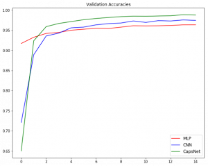
Looks even better than the previous models right? It outperforms all the architectures we saw before. The image below summarizes our experiments:

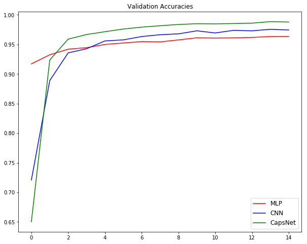
This proves that our hypothesis was correct – CapsNets are truly worth exploring!

PS – You can try experimenting this with any other dataset. If you do, please share your experience in the comments section below!

Intuition behind Capsule Networks

As with all the Deep Learning puns to understand its concepts – we will take examples of cat pictures to understand the promise (and potential) of Capsule Networks.

Let’s start with a question – which animal is depicted in the image below? (PS – I’ve already given you a hint!).

If you guessed it right, yes its a cat! But how did you know its a cat? Was it the eyes or the cuteness? We’ll break it down so that we can clarify our hypothesis.

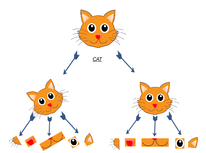
Case 1 – Simple image

So let’s say this is the cat. How did you figure out that it is a cat? One possible approach could be to break it down into individual features, such as eyes, nose, ears, etc. This idea is summarised in the image below:

So what we are essentially doing is decomposing high level features to low level ones. Concretely, you can define this as –

P(face) = P(nose) & ( 2 x P(whiskers) ) & P(mouth) & ( 2 x P(eyes) ) & ( 2 x P(ears) )

where we can define P(face) as the presence of a face of the cat in the image. Iteratively, you can also define even more low level features, like shapes and edges, in order to simplify the procedure.

Case 2 – Rotated Image

Now what if I rotate the image by 30 degrees?

If you go by the same features as we defined before, we would not be able to identify the cat. This is because the orientation of the low level features also changes. So the features which you defined previously will also change.

So now, your overall cat recognizer would probably look like this:

More specifically, you can represent this as:

P(face) = ( P(nose) & ( 2 x P(whiskers) ) & P(mouth) & ( 2 x P(eyes) ) & ( 2 x P(ears) ) )

                OR

                ( P(rotated_nose) & ( 2 x P(rotated_whiskers) ) & P(rotated_mouth) & ( 2 x
                  P(rotated_eyes) ) & ( 2 x P(rotated_ears) ) )

Case 3 : Upside Down Image

Now just to increase the complexity, what if we have a completely upside down image?

Our approach seems like a brute force search for all possible rotations of the low level features. We will need a more robust method to do the job.

Take a moment to think about a possible workaround for this before reading further. If you come up with anything that could solve this problem, please share it with the community below!

One suggestion by the researchers was to include additional properties of the low level features itself – such as rotational angle. This is how you can check not only the presence of a feature, but also its rotation. For example, see the image below:

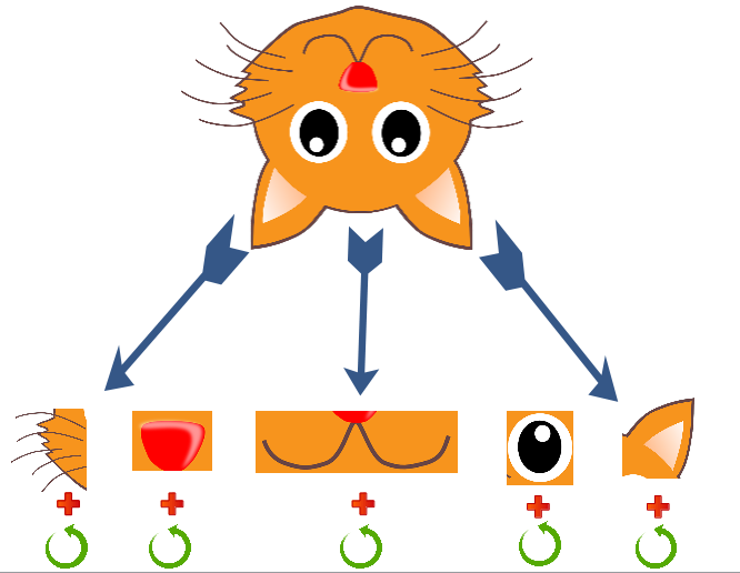
In a more rigorous way, you can define this as:

P(face) = [ P(nose), R(nose) ] & [ P(whiskers_1), R(whisker_1) ] & [ P(whiskers_2), R(whisker_2) ] & [ P(mouth), R(mouth) ] & …

where we also catch the rotational value of the individual as R() of a feature. So for this approach – change in rotational angle is represented in a meaningful way. This property is called rotational equivariance.

Food for thought – we can also scale up this idea to capture more aspects of the low level features, such as scale, stroke thickness, skew, etc. This would help us grasp an object in the image more clearly. This is how capsule networks were envisioned to work when they were designed.

Here, we saw an important aspect of Capsule Networks. Another important feature of Capsule networks is dynamic routing. We will take a look at this next.

Now let’s take a Dog vs Cat Classification problem.

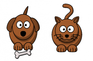
Overall, if you see them – they look very similar. But there are some significant differences in the images that can help us figure out which is the cat and which is the dog. Can you guess the difference?

As we did in the previous sub-section – we will define features in the images which will help us figure out the differences.

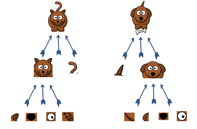
As we see in the image below, we can define iteratively complex features to come up with the solution. We can first define very low level facial features such as eyes and ears and them combine them to find a face. After that, we can combine the facial and body features to arrive at our solution, i.e, is it a dog or a cat.

Now suppose that you have a new image, with all the extracted low level features. Now you are trying to figure out the class of this image.

We picked a feature randomly and it turned out to be the eye. Can it single handedly help us figure out the class?

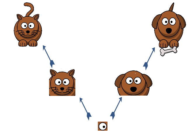
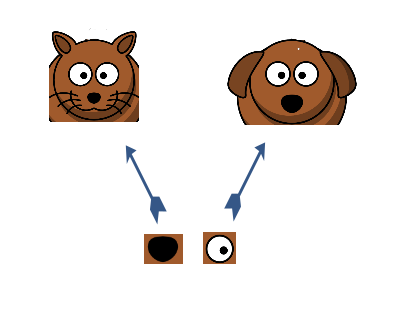
We see that eye alone is not a differentiating factor. So our next step is to add more features to our analysis. The next feature we randomly pick out is a nose. For the moment, we’ll only look at the low-level feature space and the intermediate-level feature space.

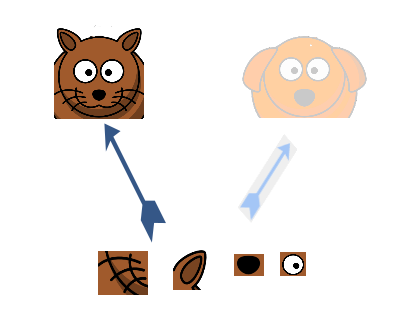
We still see that they are not enough for classification. So our next logical step will be to take all the features and combine their guess estimates of which class they will output. In the example below, we see that by combining four features – eyes, nose, ears and whiskers – we can say that it is more probable that it is a cat’s face rather than a dog’s face. So we will give more weightage to these features when we are performing cat recognition in an image. We will do this step iteratively at each feature level, so that we can “route” the correct information to those feature detectors that need the information for classification.

In simple English, we are trying to figure out that at each lower level, what will be the most probable output at its immediate higher level? Will the higher level feature activate when it gets the information from all the features? If that higher level feature will indeed activate, the lower level feature will give its information to that feature. Otherwise it will not pass on this information, as it is somewhat irrelevant for that feature detector.

In capsule terms, lower level capsule will send its input to the higher level capsule that “agrees” with its input. This is the essence of the dynamic routing algorithm.

These essentially are the most important aspects of a capsule network, which sets it apart from traditional deep learning architectures – namely equivariance and dynamic routing. The result is that a capsule network is more robust to orientation and pose of the data – and it can even train on comparatively lesser number of data points with a better performance in solving the same problem. Researchers have developed a state of the art performance of Capsule Networks on the ultra-popular MNIST dataset with a couple of hundred times less data. This is the power of Capsule network.

Of course, Capsule networks come with their own baggage – like requiring comparatively more training time and resources than most other deep learning architectures. But it is just a matter of time before we figure out how to tune them properly so that they can come out of their current research phase into production. I am eagerly waiting for that! Are you?

Code Walkthrough of CapsNet on MNIST

We will cover the first section in more depth, along with a code walkthough to get more clarity. I would recommend following along with the code on your own machine to get the maximum benefit out of it.

We will first have to clear the prerequisite data and import the libraries to set up our system. I would suggest having anaconda installed in your system, as most of the prerequisite libraries are already installed along with it.

Before we begin, you need to download the dataset from the “Identify the Digits” practice problem. Let’s take a look at our problem statement:

Our problem is an image recognition problem, to identify digits from a given 28 x 28 image. We have a subset of images for training and the rest for testing our model. The dataset contains a zipped file of all the images and both the train.csv and test.csv have the name of corresponding train and test images. Any additional features are not provided in the datasets, just the raw images are provided in ‘.png’ format.

Before starting this experiment, make sure you have Keras installed in your system. Refer to the official installation guide. We will use TensorFlow for the backend, so make sure you have this in your config file. If not, follow the steps given here.

We will then use an open source implementation of Capsule Networks by Xifeng Guo. To set it up on your system, type the below commands in the command prompt:

git clone https://github.com/XifengGuo/CapsNet-Keras.git capsnet-keras
cd capsnet-keras

You can then fire up a Jupyter notebook and follow along with the code below.

We will first import the necessary module required for our implementation.

%pylab inline
import os
import numpy as np
import pandas as pd
from scipy.misc import imread
from sklearn.metrics import accuracy_score

import tensorflow as tf
import keras
import keras.backend as K

from capsulelayers import CapsuleLayer, PrimaryCap, Length, Mask
from keras import layers, models, optimizers
from keras.preprocessing.image import ImageDataGenerator

K.set_image_data_format('channels_last')

Then, we will use a seed value for our random initialization.

# To stop potential randomness
seed = 128
rng = np.random.RandomState(seed)

The next step is to set directory paths, for safekeeping!

root_dir = os.path.abspath('.')
data_dir = os.path.join(root_dir, 'data')

Now read in our datasets. These are in ‘.csv’ format, and have a file name along with the appropriate labels.

train = pd.read_csv(os.path.join(data_dir, 'train.csv'))
test = pd.read_csv(os.path.join(data_dir, 'test.csv'))

train.head()

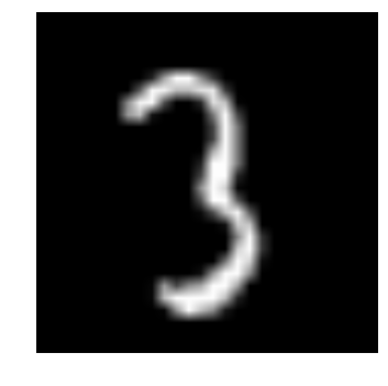
Let us see what our data looks like! We read our image and display it.

img_name = rng.choice(train.filename)
filepath = os.path.join(data_dir, 'train', img_name)

img = imread(filepath, flatten=True)

pylab.imshow(img, cmap='gray')
pylab.axis('off')
pylab.show()

Now for easier data manipulation, we’ll store all our images as numpy arrays.

temp = []
for img_name in train.filename:
   image_path = os.path.join(data_dir, 'train', img_name)
   img = imread(image_path, flatten=True)
   img = img.astype('float32')
   temp.append(img)
 
train_x = np.stack(temp)

train_x /= 255.0
train_x = train_x.reshape(-1, 784).astype('float32')

temp = []
for img_name in test.filename:
   image_path = os.path.join(data_dir, 'test', img_name)
   img = imread(image_path, flatten=True)
   img = img.astype('float32')
   temp.append(img)
 
test_x = np.stack(temp)

test_x /= 255.0
test_x = test_x.reshape(-1, 784).astype('float32')

train_y = keras.utils.np_utils.to_categorical(train.label.values)

As this is a typical ML problem, we will create a validation set to test the proper functioning of our model. Let’s take a split size of 70:30 for the train set vs. the validation set.

split_size = int(train_x.shape[0]*0.7)

train_x, val_x = train_x[:split_size], train_x[split_size:]
train_y, val_y = train_y[:split_size], train_y[split_size:]

Now comes the main part!

For our analysis, we will be building three deep learning architectures to do a comparative study (like we did in the first section of this article):

1. Multi Layer Perceptron
2. Convolutional Neural Network
3. Capsule Network

1. Multi Layer Perceptron

Let us define our neural network architecture. We define a neural network with 3 layers  input, hidden and output. The number of neurons in input and output are fixed, as the input is our 28 x 28 image and the output is a 10 x 1 vector representing the class. We take 50 neurons in the hidden layer. Here, we use Adam as our optimization algorithms, which is an efficient variant of Gradient Descent algorithm. There are a number of other optimizers available in keras (refer here). In case you don’t understand any of these terminologies, check out the article on fundamentals of neural network to know more in depth of how it works.

# define vars
input_num_units = 784
hidden_num_units = 50
output_num_units = 10

epochs = 15
batch_size = 128

# import keras modules

from keras.models import Sequential
from keras.layers import InputLayer, Convolution2D, MaxPooling2D, Flatten, Dense

# create model
model = Sequential([
 Dense(units=hidden_num_units, input_dim=input_num_units, activation='relu'),
 Dense(units=output_num_units, input_dim=hidden_num_units, activation='softmax'),
])

# compile the model with necessary attributes
model.compile(loss='categorical_crossentropy', optimizer='adam', metrics=['accuracy'])

Now that we have defined our model, we’ll print the architecture.

model.summary()

trained_model = model.fit(train_x, train_y, nb_epoch=epochs, batch_size=batch_size, validation_data=(val_x, val_y))

After training for 15 epochs, this is the output we get:

Epoch 14/15
34300/34300 [==============================] - 1s 41us/step - loss: 0.0597 - acc: 0.9834 - val_loss: 0.1227 - val_acc: 0.9635
Epoch 15/15
34300/34300 [==============================] - 1s 41us/step - loss: 0.0553 - acc: 0.9842 - val_loss: 0.1245 - val_acc: 0.9637

Pretty decent – but we can definitely improve upon this.

2. Convolutional Neural Network

But we see what a CNN can do, we have to reshape our data into a 2D format so that we can pass it on to our CNN model.

# reshape data
train_x_temp = train_x.reshape(-1, 28, 28, 1)
val_x_temp = val_x.reshape(-1, 28, 28, 1)

# define vars
input_shape = (784,)
input_reshape = (28, 28, 1)


pool_size = (2, 2)

hidden_num_units = 50
output_num_units = 10

batch_size = 128

We will now define our CNN model.

model = Sequential([
 InputLayer(input_shape=input_reshape),

Convolution2D(25, 5, 5, activation='relu'),
 MaxPooling2D(pool_size=pool_size),

Convolution2D(25, 5, 5, activation='relu'),
 MaxPooling2D(pool_size=pool_size),

Convolution2D(25, 4, 4, activation='relu'),

Flatten(),

Dense(output_dim=hidden_num_units, activation='relu'),

Dense(output_dim=output_num_units, input_dim=hidden_num_units, activation='softmax'),
])

model.compile(loss='categorical_crossentropy', optimizer='adam', metrics=['accuracy'])

#trained_model_conv = model.fit(train_x_temp, train_y, nb_epoch=epochs, batch_size=batch_size, validation_data=(val_x_temp, val_y))

model.summary()

We will also tweak our process a bit, by augmenting the data.

# Begin: Training with data augmentation ---------------------------------------------------------------------#
def train_generator(x, y, batch_size, shift_fraction=0.1):
   train_datagen = ImageDataGenerator(width_shift_range=shift_fraction,
   height_shift_range=shift_fraction) # shift up to 2 pixel for MNIST
   generator = train_datagen.flow(x, y, batch_size=batch_size)
   while 1:
     x_batch, y_batch = generator.next()
     yield ([x_batch, y_batch])
 
# Training with data augmentation. If shift_fraction=0., also no augmentation.
trained_model2 = model.fit_generator(generator=train_generator(train_x_temp, train_y, 1000, 0.1),
 steps_per_epoch=int(train_y.shape[0] / 1000),
 epochs=epochs,
 validation_data=[val_x_temp, val_y])
# End: Training with data augmentation -----------------------------------------------------------------------#

This is the result we get from our CNN model:

Epoch 14/15
34/34 [==============================] - 4s 108ms/step - loss: 0.1278 - acc: 0.9604 - val_loss: 0.0820 - val_acc: 0.9757
Epoch 15/15
34/34 [==============================] - 4s 110ms/step - loss: 0.1256 - acc: 0.9626 - val_loss: 0.0827 - val_acc: 0.9746

3. Capsule network

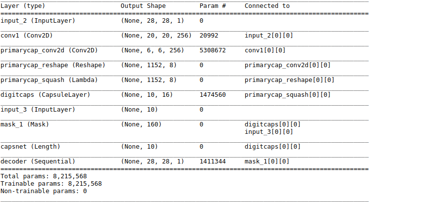
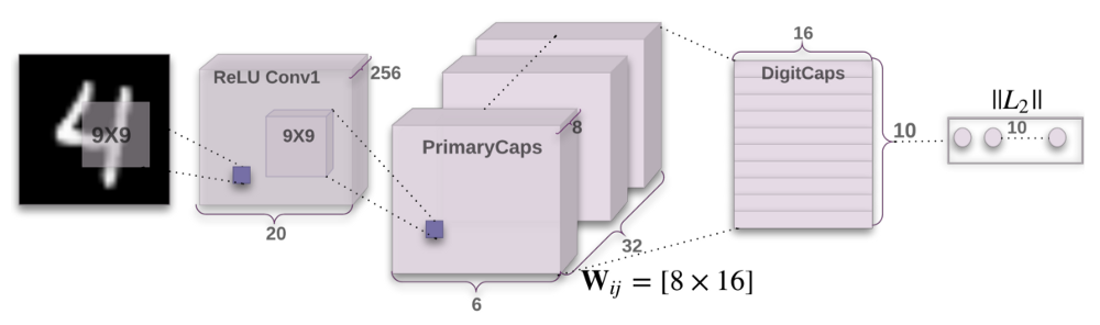
Now we will build our final architecture – Capsule network. The code is punctuated with comments if you want to understand the details. Here is how the architecture of Capsule Networks looks like:

Let’s build this model.

def CapsNet(input_shape, n_class, routings):
   """
   A Capsule Network on MNIST.
   :param input_shape: data shape, 3d, [width, height, channels]
   :param n_class: number of classes
   :param routings: number of routing iterations
   :return: Two Keras Models, the first one used for training, and the second one for evaluation.
   `eval_model` can also be used for training.
   """
   x = layers.Input(shape=input_shape)

   # Layer 1: Just a conventional Conv2D layer
   conv1 = layers.Conv2D(filters=256, kernel_size=9, strides=1, padding='valid', activation='relu', name='conv1')(x)

   # Layer 2: Conv2D layer with `squash` activation, then reshape to [None, num_capsule, dim_capsule]
   primarycaps = PrimaryCap(conv1, dim_capsule=8, n_channels=32, kernel_size=9, strides=2, padding='valid')

   # Layer 3: Capsule layer. Routing algorithm works here.
   digitcaps = CapsuleLayer(num_capsule=n_class, dim_capsule=16, routings=routings,
   name='digitcaps')(primarycaps)

   # Layer 4: This is an auxiliary layer to replace each capsule with its length. Just to match the true label's shape.
   # If using tensorflow, this will not be necessary. :)
   out_caps = Length(name='capsnet')(digitcaps)

   # Decoder network.
   y = layers.Input(shape=(n_class,))
   masked_by_y = Mask()([digitcaps, y]) # The true label is used to mask the output of capsule layer. For training
   masked = Mask()(digitcaps) # Mask using the capsule with maximal length. For prediction

   # Shared Decoder model in training and prediction
   decoder = models.Sequential(name='decoder')
   decoder.add(layers.Dense(512, activation='relu', input_dim=16*n_class))
   decoder.add(layers.Dense(1024, activation='relu'))
   decoder.add(layers.Dense(np.prod(input_shape), activation='sigmoid'))
   decoder.add(layers.Reshape(target_shape=input_shape, name='out_recon'))

   # Models for training and evaluation (prediction)
   train_model = models.Model([x, y], [out_caps, decoder(masked_by_y)])
   eval_model = models.Model(x, [out_caps, decoder(masked)])

   # manipulate model
   noise = layers.Input(shape=(n_class, 16))
   noised_digitcaps = layers.Add()([digitcaps, noise])
   masked_noised_y = Mask()([noised_digitcaps, y])
   manipulate_model = models.Model([x, y, noise], decoder(masked_noised_y))
   return train_model, eval_model, manipulate_model


def margin_loss(y_true, y_pred):
   """
   Margin loss for Eq.(4). When y_true[i, :] contains not just one `1`, this loss should work too. Not test it.
   :param y_true: [None, n_classes]
   :param y_pred: [None, num_capsule]
   :return: a scalar loss value.
   """
   L = y_true * K.square(K.maximum(0., 0.9 - y_pred)) + \
   0.5 * (1 - y_true) * K.square(K.maximum(0., y_pred - 0.1))

   return K.mean(K.sum(L, 1))

model, eval_model, manipulate_model = CapsNet(input_shape=train_x_temp.shape[1:],
 n_class=len(np.unique(np.argmax(train_y, 1))),
 routings=3)

# compile the model
model.compile(optimizer=optimizers.Adam(lr=0.001),
 loss=[margin_loss, 'mse'],
 loss_weights=[1., 0.392],
 metrics={'capsnet': 'accuracy'})

model.summary()

# Begin: Training with data augmentation ---------------------------------------------------------------------#
def train_generator(x, y, batch_size, shift_fraction=0.1):
 train_datagen = ImageDataGenerator(width_shift_range=shift_fraction,
 height_shift_range=shift_fraction) # shift up to 2 pixel for MNIST
 generator = train_datagen.flow(x, y, batch_size=batch_size)
 while 1:
 x_batch, y_batch = generator.next()
 yield ([x_batch, y_batch], [y_batch, x_batch])

# Training with data augmentation. If shift_fraction=0., also no augmentation.
trained_model3 = model.fit_generator(generator=train_generator(train_x_temp, train_y, 1000, 0.1),
 steps_per_epoch=int(train_y.shape[0] / 1000),
 epochs=epochs)
# End: Training with data augmentation -----------------------------------------------------------------------#

This is the result we get from our CapsNet model:

Epoch 14/15
34/34 [==============================] - 108s 3s/step - loss: 0.0445 - capsnet_loss: 0.0218 - decoder_loss: 0.0579 - capsnet_acc: 0.9846 - val_loss: 0.0364 - val_capsnet_loss: 0.0159 - val_decoder_loss: 0.0522 - val_capsnet_acc: 0.9887
Epoch 15/15
34/34 [==============================] - 107s 3s/step - loss: 0.0423 - capsnet_loss: 0.0201 - decoder_loss: 0.0567 - capsnet_acc: 0.9859 - val_loss: 0.0362 - val_capsnet_loss: 0.0162 - val_decoder_loss: 0.0510 - val_capsnet_acc: 0.9880

To summarize, we can plot a graph of validation accuracies.

plt.figure(figsize=(10, 8))
plt.plot(trained_model.history['val_acc'], 'r', trained_model2.history['val_acc'], 'b', trained_model3.history['val_capsnet_acc'], 'g')
plt.legend(('MLP', 'CNN', 'CapsNet'),
 loc='lower right', fontsize='large')
plt.title('Validation Accuracies')
plt.show()

This ends our tryst with CapsNet!

End Notes

In this article, we went though a non-technical brief overview of capsule networks, and then went on to understand what are the most important aspects of it. We also covered CapsNet in detail, along with a code walkthrough on a Digit Recognition dataset.

I hope this article helped you grasp the concepts of CapsNet so you can implement it in your own real life use cases. If you do, please share your experience with us in the comments below.

Participate in the McKinsey Analytics Online Hackathon to win an all-expenses paid trip to an international analytics conference!

JalFaizy Shaikh 15 May 2020

Faizan is a Data Science enthusiast and a Deep learning rookie. A recent Comp. Sc. undergrad, he aims to utilize his skills to push the boundaries of AI research.