Essentials of Deep Learning: Introduction to Unsupervised Deep Learning (with Python codes)
Introduction
In one of the early projects, I was working with the Marketing Department of a bank. The Marketing Director called me for a meeting. The subject said – “Data Science Project”. I was excited, completely charged and raring to go. I was hoping to get a specific problem, where I could apply my data science wizardry and benefit my customer.
The meeting started on time. The Director said “Please use all the data we have about our customers and tell us the insights about our customers, which we don’t know. We really want to use data science to improve our business.”
I was left thinking “What insights do I present to the business?”
Data scientists use a variety of machine learning algorithms to extract actionable insights from the data they’re provided. The majority of them are supervised learning problems, because you already know what you are required to predict. The data you are given comes with a lot of details to help you reach your end goal.
Source: danielmiessler
On the other hand, unsupervised learning is a complex challenge. But it’s advantages are numerous. It has the potential to unlock previously unsolvable problems and has gained a lot of traction in the machine learning and deep learning community.
I am planning to write a series of articles focused on Unsupervised Deep Learning applications. This article specifically aims to give you an intuitive introduction to what the topic entails, along with an application of a real life problem. In the next few articles, I will focus more on the internal workings of the techniques involved in deep learning.
Note – This article assumes a basic knowledge of Deep Learning and Machine learning concepts. If you want to brush up on them, you can go through these resources:
- Experiments With Data Course
- Introduction to Data Science Course
- Fundamentals of Deep Learning – Starting with Artificial Neural Network
So let’s get started!
Table of Contents
- Why Unsupervised Learning?
- Case Study of Unsupervised Deep Learning
- Defining our Problem – How to Organize a Photo Gallery?
- Approach 1 – Arrange on the basis of time
- Approach 2 – Arrange on the basis of location
- Approach 3 – Extract Semantic meaning from the image and use it organize the photos
- Code Walkthrough of Unsupervised Deep Learning on the MNIST dataset
Why Unsupervised Learning?
A typical workflow in a machine learning project is designed in a supervised manner. We tell the algorithm what to do and what not to do. This generally gives a structure for solving a problem, but it limits the potential of that algorithm in two ways:
- It is bound by the biases in which it is being supervised in. Of course it learns how to perform that task on its own. But it is prohibited to think of other corner cases that could occur when solving the problem.
- As the learning is supervised – there is a huge manual effort involved in creating the labels for our algorithm. So fewer the manual labels you create, less is the training that you can perform for your algorithm.
To solve this issue in an intelligent way, we can use unsupervised learning algorithms. These algorithms derive insights directly from the data itself, and work as summarizing the data or grouping it, so that we can use these insights to make data driven decisions.
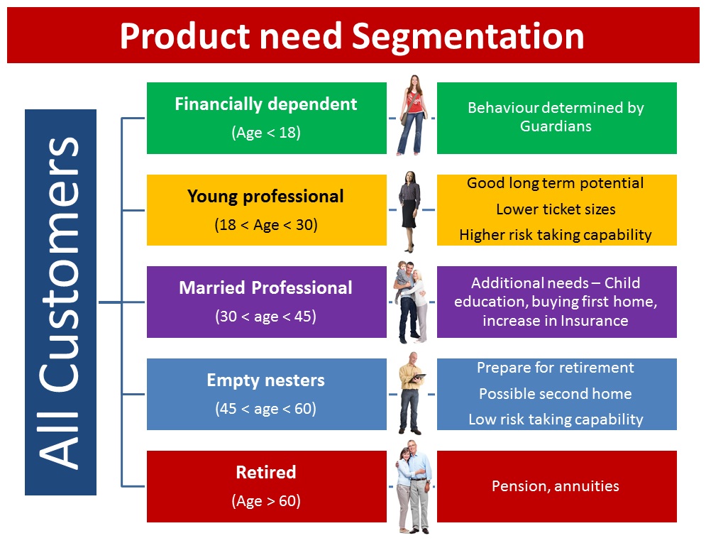
Let’s take an example to better understand this concept. Let’s say a bank wants to divide its customers so that they can recommend the right products to them. They can do this in a data-driven way – by segmenting the customers on the basis of their ages and then deriving insights from these segments. This would help the bank give better product recommendations to their customers, thus increasing customer satisfaction.
Case Study of Unsupervised Deep Learning
In this article, we will take a look at a case study of unsupervised learning on unstructured data. As you might be aware, Deep Learning techniques are usually most impactful where a lot of unstructured data is present. So we will take an example of Deep Learning being applied to the Image Processing domain to understand this concept.
Defining our Problem – How to Organize a Photo Gallery?
I have 2000+ photos in my smartphone right now. If I had been a selfie freak, the photo count would easily be 10 times more. Sifting through these photos is a nightmare, because every third photo turns out to be unnecessary and useless for me. I’m sure most of you will be able to relate to my plight!
Ideally, what I would want is an app which organizes the photos in such a manner that I can go through most of the photos and have a peek at it if I want. This would actually give me context as such of the different kinds of photos I have right now.
To get a clearer perspective of the problem, I went through my mobile and tried to identify the categories of the images by myself. Here are the insights I gathered:
- First and foremost, I found that one-third of my photo gallery is filled with memes (Thanks to my lovely friends on WhatsApp).
- I personally collect interesting quotes / shares I come across on Reddit. These are mostly motivational or funny, depending on which subreddit I downloaded them from.
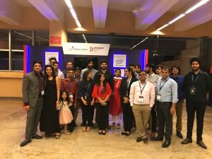
- There are at least 200 images I captured, or my colleagues shared, of the famous DataHack Summit and the subsequent AV outing we had in Kerala
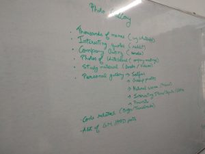
- There are a few photos of whiteboard discussions that happen frequently during meetings.
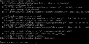
- Then there are a few images/screenshots of code tracebacks/bugs that require internal team discussions. They are a necessary evil that has to be purged after use.
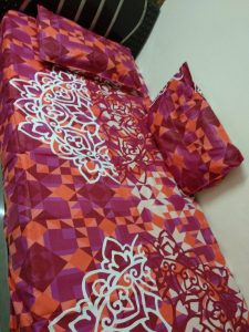
- I also found dispersed “private & personal” images, such as selfies, group photos and a few objects/sceneries. They are few, but they are my prized possessions.
- Last but not the least – there were numerous “good morning”, “happy birthday” and “happy diwali” posts that I desperately want to delete from my gallery. No matter how much I exterminate them, they just keep coming back!

Now that you know the scenerio, can you think of the different ways to better organize my photos through an automated algorithm? You can discuss your thoughts on this discussion thread.
In the below sections, we will discuss a few approaches I have come up with to solve this problem.
Approach 1 – Arrange on the basis of time
The simplest way is to arrange the photos on the basis of time. Each day could have a different folder for itself. Typically, most of the photo viewing apps use this approach (eg. Google Photos app).

The upside of this will be that all the events that happened on that day will be stored together. The downside of this approach is that it is too generic. Each day, I could have photos that are from an outing, or a motivational quote, etc. Both of them will be mixed together – which defeats the purpose altogether.
Approach 2 – Arrange on the basis of location
A comparatively better approach would be to arrange the photos based on where they were taken. So, for example, with each camera click we would capture where the image was taken. Then we can make folders on the basis of these locations – either country/city wise or locality wise, depending on the granularity we want. This approach is also being used by most photo apps.
The downside of this approach is the simplistic idea on which it was created. How can we define the location of a meme, or a cartoon – which takes a fair share of my image gallery? So this approach lacks ingenuity as well.
Approach 3 – Extract Semantic meaning from the image and use it to define my collection
The approaches we have seen so far were mostly dependent on the metadata that is captured along with the image. A better way to organize the photos would be to extract semantic information from the image itself and use that information intelligently.
Let’s break this idea down into parts. Suppose we have a similar variety of photos (as mentioned above). What trends should our algorithm capture?
- Is the captured image of a natural scene or is it an artificially generated image?
- Is there textual material in the photograph? If there is – can we identify what it is?
- What are the different kinds of objects present in the photograph? Do they combine to define the aesthetics of the image?
- Are there people present in the photograph? Can we recognize them?
- Are there similar images on the web which can help us identify the context of the image?
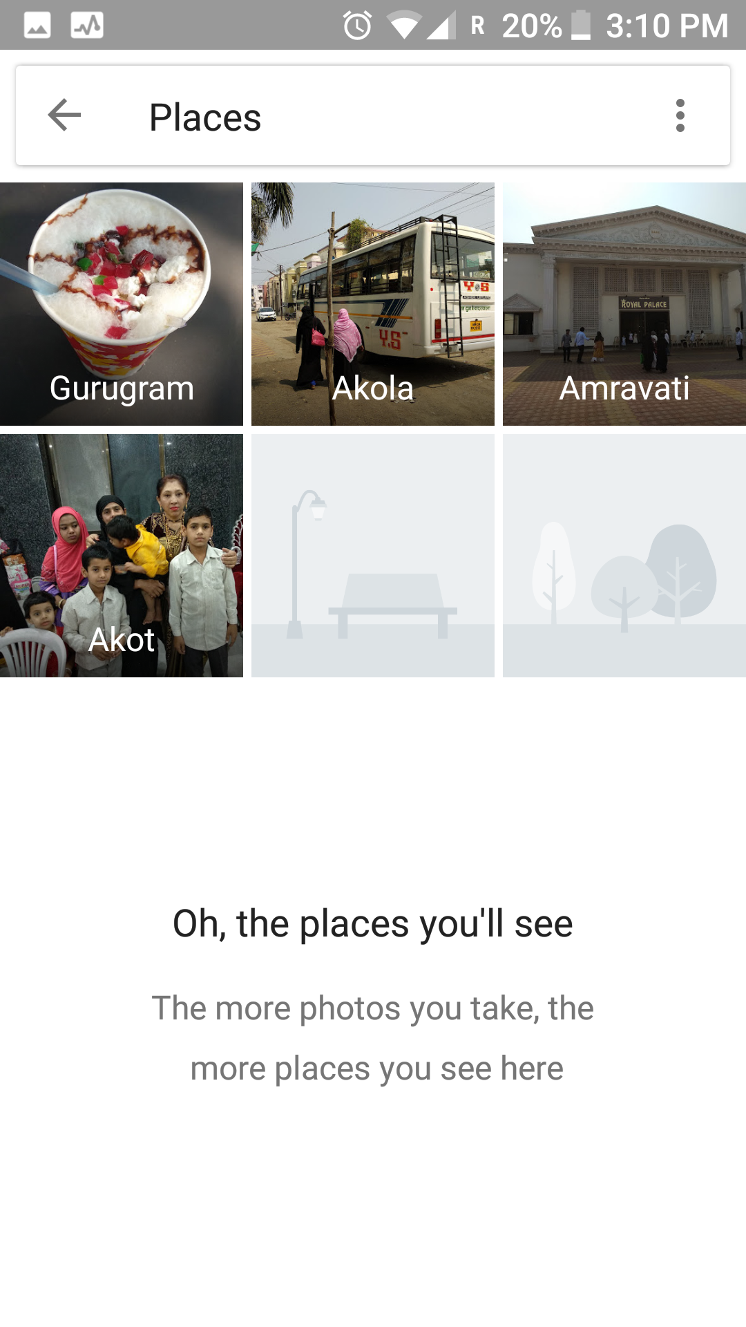
So our algorithm should ideally capture this information without explicitly tagging what is present and what is not, and use it to organize and segment our photos. Ideally, our final organized app could look like this:

This approach is what we call an “unsupervised way” to solve problems. We did not directly define the outcome that we want. Instead, we trained an algorithm to find those outcomes for us! Our algorithm summarizes the data in an intelligent manner, and then tries to solve the problem on the basis of these inferences. Pretty cool, right?
Now you may be wondering – how can we leverage Deep Learning for unsupervised learning problems?
As we saw in the case study above, by extracting semantic information from the image, we can get a better view of the similarity of images. Thus, our problem can be formulated as – how can we reduce the dimensions of an image so that we can reconstruct the image back from these encoded representations?
Here, we can use a deep learning architecture called Auto Encoders.
Let me give you a high level overview of Auto Encoders. The idea behind using this algorithm is that you are training it to recreate what it just learnt. But the catch is that it has to use a much smaller representation phase to recreate it.
For example, an Auto Encoder with encoding set to 10 is trained on images of cats, each of size 100×100. So the input dimension is 10,000, and the Auto Encoder has to represent all this information in a vector of size 10 (as seen in the image below).
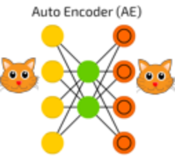
An auto encoder can be logically divided into two parts: an encoder and a decoder. The task of the encoder is to convert the input to a lower dimensional representation, while the task of the decoder is to recreate the input from this lower dimensional representation.
This was a very high level overview of auto encoders. In the next article – we will look at them in more detail.
Note – This is more of a forewarning; but the current state-of-the-art methods still aren’t mature enough to handle industry level problems with ease. Although research in this field is booming, it would take a few more years for our algorithms to become “industrially accepted”.
Code Walkthrough of Unsupervised Deep Learning on MNIST data
Now that you have an intuition of solving unsupervised learning problems using deep learning – we will apply our knowledge on a real life problem. Here, we will take an example of the MNIST dataset – which is considered as the go-to dataset when trying our hand on deep learning problems. Let us understand the problem statement before jumping into the code.
The original problem statement is to identify individual digits from an image. You are given the labels of the digit that the image contains. But for our case study, we will try to figure out which of the images are similar to each other and cluster them into groups. As a proxy, we will check the purity of these groups by inspecting their labels. You can find the data on AV’s DataHack platform – the Identify the Digits practice problem.
We will perform three Unsupervised Learning techniques and check their performance, namely:
- KMeans directly on image
- KMeans + Autoencoder (a simple deep learning architecture)
- Deep Embedded Clustering algorithm (advanced deep learning)
We will look into the details of these algorithms in another article. For the purposes of this post, let’s see how we can attempt to solve this problem.
Before starting this experiment, make sure you have Keras installed in your system. Refer to the official installation guide. We will use TensorFlow for the backend, so make sure you have this in your config file. If not, follow the steps given here.
We will then use an open source implementation of DEC algorithm by Xifeng Guo. To set it up on your system, type the below commands in the command prompt:
git clone https://github.com/XifengGuo/DEC-keras
cd DEC-keras
You can then fire up a Jupyter notebook and follow along with the code below.
First we will import all the necessary modules for our code walkthrough.
%pylab inline
import os
import keras
import metrics
import numpy as np
import pandas as pd
import keras.backend as K

from time import time

from keras import callbacks
from keras.models import Model
from keras.optimizers import SGD
from keras.layers import Dense, Input
from keras.initializers import VarianceScaling
from keras.engine.topology import Layer, InputSpec

from scipy.misc import imread
from sklearn.cluster import KMeans
from sklearn.metrics import accuracy_score, normalized_mutual_info_score
# To stop potential randomness
seed = 128
rng = np.random.RandomState(seed)
root_dir = os.path.abspath('.')
data_dir = os.path.join(root_dir, 'data', 'mnist')
Read the train and test files.
train = pd.read_csv(os.path.join(data_dir, 'train.csv'))
test = pd.read_csv(os.path.join(data_dir, 'test.csv'))

train.head()
Note that in this dataset, you have also been given the labels for each image. This is generally not seen in an unsupervised learning scenario. Here, we will use these labels to evaluate how our unsupervised learning models perform.
Now let us plot an image to view what our data looks like.
img_name = rng.choice(train.filename)
filepath = os.path.join(data_dir, 'train', img_name)

img = imread(filepath, flatten=True)

pylab.imshow(img, cmap='gray')
pylab.axis('off')
pylab.show()

temp = []
for img_name in train.filename:
    image_path = os.path.join(data_dir, 'train', img_name)
    img = imread(image_path, flatten=True)
    img = img.astype('float32')
    temp.append(img)

train_x = np.stack(temp)

train_x /= 255.0
train_x = train_x.reshape(-1, 784).astype('float32')

temp = []
for img_name in test.filename:
    image_path = os.path.join(data_dir, 'test', img_name)
    img = imread(image_path, flatten=True)
    img = img.astype('float32')
    temp.append(img)

test_x = np.stack(temp)

test_x /= 255.0
test_x = test_x.reshape(-1, 784).astype('float32')
train_y = train.label.values
split_size = int(train_x.shape[0]*0.7)

train_x, val_x = train_x[:split_size], train_x[split_size:]
train_y, val_y = train_y[:split_size], train_y[split_size:]
km = KMeans(n_jobs=-1, n_clusters=10, n_init=20)
km.fit(train_x)
pred = km.predict(val_x)
Mutual information is a symmetric measure for the degree of dependency between the clustering and the manual classification. It is based on the notion of cluster purity pi, which measures the quality of a single cluster Ci, the largest number of objects in cluster Ci which Ci has in common with a manual class Mj, having compared Ci to all manual classes in M. Because NMI is normalized, we can use it to compare clusterings with different numbers of clusters.
The formula for NMI is:
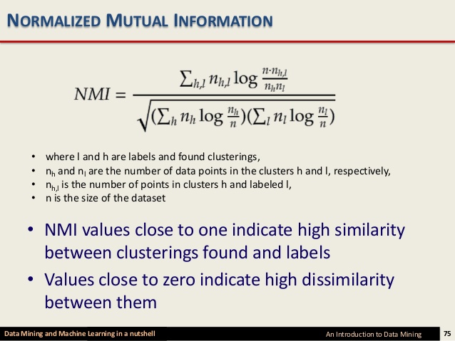
Source: Slideshare
normalized_mutual_info_score(val_y, pred)
# this is our input placeholder
input_img = Input(shape=(784,))

# "encoded" is the encoded representation of the input
encoded = Dense(500, activation='relu')(input_img)
encoded = Dense(500, activation='relu')(encoded)
encoded = Dense(2000, activation='relu')(encoded)
encoded = Dense(10, activation='sigmoid')(encoded)

# "decoded" is the lossy reconstruction of the input
decoded = Dense(2000, activation='relu')(encoded)
decoded = Dense(500, activation='relu')(decoded)
decoded = Dense(500, activation='relu')(decoded)
decoded = Dense(784)(decoded)

# this model maps an input to its reconstruction
autoencoder = Model(input_img, decoded)
autoencoder.summary()
#  this model maps an input to its encoded representation
encoder = Model(input_img, encoded)
autoencoder.compile(optimizer='adam', loss='mse')
pred_auto_train = encoder.predict(train_x)
pred_auto = encoder.predict(val_x)
km.fit(pred_auto_train)
pred = km.predict(pred_auto)
normalized_mutual_info_score(val_y, pred)
"""
Keras implementation for Deep Embedded Clustering (DEC) algorithm:

Original Author:
    Xifeng Guo. 2017.1.30
"""


def autoencoder(dims, act='relu', init='glorot_uniform'):
    """
    Fully connected auto-encoder model, symmetric.
    Arguments:
        dims: list of number of units in each layer of encoder. dims[0] is input dim, dims[-1] is units in hidden layer.
            The decoder is symmetric with encoder. So number of layers of the auto-encoder is 2*len(dims)-1
        act: activation, not applied to Input, Hidden and Output layers
    return:
        (ae_model, encoder_model), Model of autoencoder and model of encoder
    """
    n_stacks = len(dims) - 1
    # input
    x = Input(shape=(dims[0],), name='input')
    h = x

    # internal layers in encoder
    for i in range(n_stacks-1):
        h = Dense(dims[i + 1], activation=act, kernel_initializer=init, name='encoder_%d' % i)(h)

    # hidden layer
    h = Dense(dims[-1], kernel_initializer=init, name='encoder_%d' % (n_stacks - 1))(h)  # hidden layer, features are extracted from here

    y = h
    # internal layers in decoder
    for i in range(n_stacks-1, 0, -1):
        y = Dense(dims[i], activation=act, kernel_initializer=init, name='decoder_%d' % i)(y)

    # output
    y = Dense(dims[0], kernel_initializer=init, name='decoder_0')(y)

    return Model(inputs=x, outputs=y, name='AE'), Model(inputs=x, outputs=h, name='encoder')


class ClusteringLayer(Layer):
    """
    Clustering layer converts input sample (feature) to soft label, i.e. a vector that represents the probability of the
    sample belonging to each cluster. The probability is calculated with student's t-distribution.

    # Example
    ```
        model.add(ClusteringLayer(n_clusters=10))
    ```
    # Arguments
        n_clusters: number of clusters.
        weights: list of Numpy array with shape `(n_clusters, n_features)` witch represents the initial cluster centers.
        alpha: parameter in Student's t-distribution. Default to 1.0.
    # Input shape
        2D tensor with shape: `(n_samples, n_features)`.
    # Output shape
        2D tensor with shape: `(n_samples, n_clusters)`.
    """

    def __init__(self, n_clusters, weights=None, alpha=1.0, **kwargs):
        if 'input_shape' not in kwargs and 'input_dim' in kwargs:
            kwargs['input_shape'] = (kwargs.pop('input_dim'),)
        super(ClusteringLayer, self).__init__(**kwargs)
        self.n_clusters = n_clusters
        self.alpha = alpha
        self.initial_weights = weights
        self.input_spec = InputSpec(ndim=2)

    def build(self, input_shape):
        assert len(input_shape) == 2
        input_dim = input_shape[1]
        self.input_spec = InputSpec(dtype=K.floatx(), shape=(None, input_dim))
        self.clusters = self.add_weight((self.n_clusters, input_dim), initializer='glorot_uniform', name='clusters')
        if self.initial_weights is not None:
            self.set_weights(self.initial_weights)
            del self.initial_weights
        self.built = True

    def call(self, inputs, **kwargs):
        """ student t-distribution, as same as used in t-SNE algorithm.
                 q_ij = 1/(1+dist(x_i, u_j)^2), then normalize it.
        Arguments:
            inputs: the variable containing data, shape=(n_samples, n_features)
        Return:
            q: student's t-distribution, or soft labels for each sample. shape=(n_samples, n_clusters)
        """
        q = 1.0 / (1.0 + (K.sum(K.square(K.expand_dims(inputs, axis=1) - self.clusters), axis=2) / self.alpha))
        q **= (self.alpha + 1.0) / 2.0
        q = K.transpose(K.transpose(q) / K.sum(q, axis=1))
        return q

    def compute_output_shape(self, input_shape):
        assert input_shape and len(input_shape) == 2
        return input_shape[0], self.n_clusters

    def get_config(self):
        config = {'n_clusters': self.n_clusters}
        base_config = super(ClusteringLayer, self).get_config()
        return dict(list(base_config.items()) + list(config.items()))


class DEC(object):
    def __init__(self,
                 dims,
                 n_clusters=10,
                 alpha=1.0,
                 init='glorot_uniform'):

        super(DEC, self).__init__()

        self.dims = dims
        self.input_dim = dims[0]
        self.n_stacks = len(self.dims) - 1

        self.n_clusters = n_clusters
        self.alpha = alpha
        self.autoencoder, self.encoder = autoencoder(self.dims, init=init)

        # prepare DEC model
        clustering_layer = ClusteringLayer(self.n_clusters, name='clustering')(self.encoder.output)
        self.model = Model(inputs=self.encoder.input, outputs=clustering_layer)

    def pretrain(self, x, y=None, optimizer='adam', epochs=200, batch_size=256, save_dir='results/temp'):
        print('...Pretraining...')
        self.autoencoder.compile(optimizer=optimizer, loss='mse')

        csv_logger = callbacks.CSVLogger(save_dir + '/pretrain_log.csv')
        cb = [csv_logger]
        if y is not None:
            class PrintACC(callbacks.Callback):
                def __init__(self, x, y):
                    self.x = x
                    self.y = y
                    super(PrintACC, self).__init__()

                def on_epoch_end(self, epoch, logs=None):
                    if epoch % int(epochs/10) != 0:
                        return
                    feature_model = Model(self.model.input,
                                          self.model.get_layer(
                                              'encoder_%d' % (int(len(self.model.layers) / 2) - 1)).output)
                    features = feature_model.predict(self.x)
                    km = KMeans(n_clusters=len(np.unique(self.y)), n_init=20, n_jobs=4)
                    y_pred = km.fit_predict(features)
                    # print()
                    print(' '*8 + '|==>  acc: %.4f,  nmi: %.4f  <==|'
                          % (metrics.acc(self.y, y_pred), metrics.nmi(self.y, y_pred)))

            cb.append(PrintACC(x, y))

        # begin pretraining
        t0 = time()
        self.autoencoder.fit(x, x, batch_size=batch_size, epochs=epochs, callbacks=cb)
        print('Pretraining time: ', time() - t0)
        self.autoencoder.save_weights(save_dir + '/ae_weights.h5')
        print('Pretrained weights are saved to %s/ae_weights.h5' % save_dir)
        self.pretrained = True

    def load_weights(self, weights):  # load weights of DEC model
        self.model.load_weights(weights)

    def extract_features(self, x):
        return self.encoder.predict(x)

    def predict(self, x):  # predict cluster labels using the output of clustering layer
        q = self.model.predict(x, verbose=0)
        return q.argmax(1)

    @staticmethod
    def target_distribution(q):
        weight = q ** 2 / q.sum(0)
        return (weight.T / weight.sum(1)).T

    def compile(self, optimizer='sgd', loss='kld'):
        self.model.compile(optimizer=optimizer, loss=loss)

    def fit(self, x, y=None, maxiter=2e4, batch_size=256, tol=1e-3,
            update_interval=140, save_dir='./results/temp'):

        print('Update interval', update_interval)
        save_interval = x.shape[0] / batch_size * 5  # 5 epochs
        print('Save interval', save_interval)

        # Step 1: initialize cluster centers using k-means
        t1 = time()
        print('Initializing cluster centers with k-means.')
        kmeans = KMeans(n_clusters=self.n_clusters, n_init=20)
        y_pred = kmeans.fit_predict(self.encoder.predict(x))
        y_pred_last = np.copy(y_pred)
        self.model.get_layer(name='clustering').set_weights([kmeans.cluster_centers_])

        # Step 2: deep clustering
        # logging file
        import csv
        logfile = open(save_dir + '/dec_log.csv', 'w')
        logwriter = csv.DictWriter(logfile, fieldnames=['iter', 'acc', 'nmi', 'ari', 'loss'])
        logwriter.writeheader()

        loss = 0
        index = 0
        index_array = np.arange(x.shape[0])
        for ite in range(int(maxiter)):
            if ite % update_interval == 0:
                q = self.model.predict(x, verbose=0)
                p = self.target_distribution(q)  # update the auxiliary target distribution p

                # evaluate the clustering performance
                y_pred = q.argmax(1)
                if y is not None:
                    acc = np.round(metrics.acc(y, y_pred), 5)
                    nmi = np.round(metrics.nmi(y, y_pred), 5)
                    ari = np.round(metrics.ari(y, y_pred), 5)
                    loss = np.round(loss, 5)
                    logdict = dict(iter=ite, acc=acc, nmi=nmi, ari=ari, loss=loss)
                    logwriter.writerow(logdict)
                    print('Iter %d: acc = %.5f, nmi = %.5f, ari = %.5f' % (ite, acc, nmi, ari), ' ; loss=', loss)

                # check stop criterion
                delta_label = np.sum(y_pred != y_pred_last).astype(np.float32) / y_pred.shape[0]
                y_pred_last = np.copy(y_pred)
                if ite > 0 and delta_label < tol:
                    print('delta_label ', delta_label, '< tol ', tol)
                    print('Reached tolerance threshold. Stopping training.')
                    logfile.close()
                    break

            # train on batch
            # if index == 0:
            #     np.random.shuffle(index_array)
            idx = index_array[index * batch_size: min((index+1) * batch_size, x.shape[0])]
            self.model.train_on_batch(x=x[idx], y=p[idx])
            index = index + 1 if (index + 1) * batch_size <= x.shape[0] else 0

            # save intermediate model
            if ite % save_interval == 0:
                print('saving model to:', save_dir + '/DEC_model_' + str(ite) + '.h5')
                self.model.save_weights(save_dir + '/DEC_model_' + str(ite) + '.h5')

            ite += 1

        # save the trained model
        logfile.close()
        print('saving model to:', save_dir + '/DEC_model_final.h5')
        self.model.save_weights(save_dir + '/DEC_model_final.h5')

        return y_pred


# setting the hyper parameters
init = 'glorot_uniform'
pretrain_optimizer = 'adam'
dataset = 'mnist'
batch_size = 2048
maxiter = 2e4
tol = 0.001
save_dir = 'results'

import os
if not os.path.exists(save_dir):
    os.makedirs(save_dir)

update_interval = 200
pretrain_epochs = 500
init = VarianceScaling(scale=1. / 3., mode='fan_in',
                       distribution='uniform')  # [-limit, limit], limit=sqrt(1./fan_in)
#pretrain_optimizer = SGD(lr=1, momentum=0.9)


# prepare the DEC model
dec = DEC(dims=[train_x.shape[-1], 500, 500, 2000, 10], n_clusters=10, init=init)

dec.pretrain(x=train_x, y=train_y, optimizer=pretrain_optimizer,
             epochs=pretrain_epochs, batch_size=batch_size,
             save_dir=save_dir)
dec.model.summary()
dec.compile(optimizer=SGD(0.01, 0.9), loss='kld')
y_pred = dec.fit(train_x, y=train_y, tol=tol, maxiter=maxiter, batch_size=batch_size,
                 update_interval=update_interval, save_dir=save_dir)
pred_val = dec.predict(val_x)
normalized_mutual_info_score(val_y, pred_val)
End Notes
In this article, we saw an overview of the concept of unsupervised deep learning with an intuitive case study. In the next series of articles, we will get into the details of how we can use these techniques to solve more real life problems.
If you have any comments / suggestions, feel free to reach out to me below!
Learn, compete, hack and get hired!
Faizan is a Data Science enthusiast and a Deep learning rookie. A recent Comp. Sc. undergrad, he aims to utilize his skills to push the boundaries of AI research.


Getting this error. What to do? Anaconda3\lib\site-packages\IPython\core\magics\pylab.py:160: UserWarning: pylab import has clobbered these variables: ['imread', 'time'] `%matplotlib` prevents importing * from pylab and numpy "\n`%matplotlib` prevents importing * from pylab and numpy"
Hi Sanjoy - that is actually not an error, but a warning. You can ignore that for now.
Thank you so much Faizan. Very helpful . unsuervised approach through Neuralnets and NMI are new to me . Possibly there are few areas i didn't understood , but needs some research on the topic . Will get back to you for any help . Thanks Again .... Can you share some article on Sequence learning as well ? may be in coming days. Thanks
Hey Chandu - you can refer this article for an intuitive guide to sequence learning (https://www.analyticsvidhya.com/blog/2018/04/sequence-modelling-an-introduction-with-practical-use-cases/) You can find many such guides on Analytics Vidhya, just a click away!
Getting this error also: C:\Users\user\Anaconda3\lib\site-packages\ipykernel_launcher.py:4: DeprecationWarning: `imread` is deprecated! `imread` is deprecated in SciPy 1.0.0, and will be removed in 1.2.0. Use ``imageio.imread`` instead. after removing the cwd from sys.path.
This is the same case as previous one, you can ignore the warning for now
In the Keras implementation for Deep Embedded Clustering (DEC) algorithm, getting this following attribute error (it ran first epoch, then the error came): --------------------------------------------------------------------------- AttributeError Traceback (most recent call last) in () 273 dec.pretrain(x=train_x, y=train_y, optimizer=pretrain_optimizer, 274 epochs=pretrain_epochs, batch_size=batch_size, --> 275 save_dir=save_dir) in pretrain(self, x, y, optimizer, epochs, batch_size, save_dir) 152 # begin pretraining 153 t0 = time() --> 154 self.autoencoder.fit(x, x, batch_size=batch_size, epochs=epochs, callbacks=cb) 155 print('Pretraining time: ', time() - t0) 156 self.autoencoder.save_weights(save_dir + '/ae_weights.h5') ~\Anaconda3\lib\site-packages\keras\engine\training.py in fit(self, x, y, batch_size, epochs, verbose, callbacks, validation_split, validation_data, shuffle, class_weight, sample_weight, initial_epoch, steps_per_epoch, validation_steps, **kwargs) 1703 initial_epoch=initial_epoch, 1704 steps_per_epoch=steps_per_epoch, -> 1705 validation_steps=validation_steps) 1706 1707 def evaluate(self, x=None, y=None, ~\Anaconda3\lib\site-packages\keras\engine\training.py in _fit_loop(self, f, ins, out_labels, batch_size, epochs, verbose, callbacks, val_f, val_ins, shuffle, callback_metrics, initial_epoch, steps_per_epoch, validation_steps) 1254 for l, o in zip(out_labels, val_outs): 1255 epoch_logs['val_' + l] = o -> 1256 callbacks.on_epoch_end(epoch, epoch_logs) 1257 if callback_model.stop_training: 1258 break ~\Anaconda3\lib\site-packages\keras\callbacks.py in on_epoch_end(self, epoch, logs) 75 logs = logs or {} 76 for callback in self.callbacks: ---> 77 callback.on_epoch_end(epoch, logs) 78 79 def on_batch_begin(self, batch, logs=None): in on_epoch_end(self, epoch, logs) 146 # print() 147 print(' '*8 + '|==> acc: %.4f, nmi: %.4f 148 % (metrics.acc(self.y, y_pred), metrics.nmi(self.y, y_pred))) 149 150 cb.append(PrintACC(x, y)) AttributeError: module 'metrics' has no attribute 'acc' In [ ]:
Hey - Thanks for spotting it out. There were a few installation steps that needed to be updated in the article. More specifically, setup of this repo is required to run the code. Please refer the steps as mentioned in the article
Great post ! Very good explanation. Have you tried denoising autoencoder ? Thanks for the blog
Hi Faizan, thanks a lot for the nice tutorial. I am not able to read the train.csv and test.csv files: there is no directory called data/mnist in the DEC-keras package I downloaded from gitub. Can you please advice on this? Thanks, Elisa
Thank you very much for your article. It is a great one and I learned a lot from it. Where can I download your code? Do I have to copy and paste into a Jupyter notebook?
Hi, You can copy and paste the code into Jupyter Notebook to run it.