Master Maximum Likelihood Estimation in R: A Step-by-Step Guide

Introduction

Interpreting how a model works is one of the most basic yet critical aspects of data science or any case study or data analysis. You build a machine learning model which is giving you pretty impressive results, but what was the process behind it? As a data scientist, you need to have an answer to this oft-asked question.

For example, let’s say you want to build a real-world model to predict the stock price of a company, and you want to build a methodology for it, but you observed that the stock price increased rapidly overnight. There could be multiple reasons behind it. Finding the likelihood estimators or unbiased estimators is the most probable reason is what Maximum Likelihood Estimation is all about. This concept is used in economics, MRIs, and satellite imaging, among other things.

Source: YouTube

In this post, we will step by step look into how Maximum Likelihood Estimation (referred to as MLE hereafter) works and how it can be used to determine coefficients or model parameters with any distribution. Understanding MLE would involve knowledge of probability value (p-value), but I will try to make it easier with examples.

Learning Objectives

• In this tutorial, we will learn about Maximum Likelihood Estimation and learn about it with an example.
• We will also learn the implementation of MLE in R.

Note: As mentioned, this article assumes that you know the basics of maths and probability. You can refresh your concepts by going through this article first – 6 Common Probability Distributions every data science professional should know.

Why Should I Use Maximum Likelihood Estimation (MLE)?

Let us say we want to predict the sale of tickets for an event. The data has the following histogram and density.

How would you model such a variable (var)? The variable is not normally distributed and is asymmetric hence it violates the assumptions of linear regression. A popular way is to transform the variable with log, sqrt, reciprocal, etc. so that the transformed variable is normally distributed and can be modeled with linear regression.

Let’s try these transformations and see how the results are:

With Log Transformation: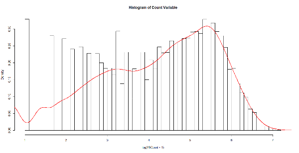

With Square Root Transformation: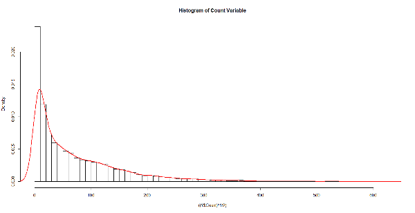

With Reciprocal: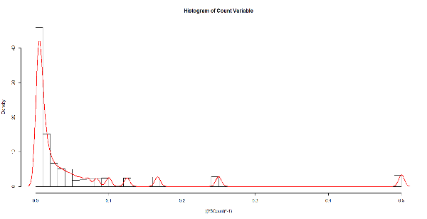

None of these is close to a normal distribution. How should we model such data so that the basic assumptions of the model are not violated? How about modeling this data with a different distribution rather than a normal one? If we do use a different distribution, how will we estimate the coefficients?

This is where Maximum Likelihood Estimation (MLE) has such a major advantage.

Understanding MLE With an Example

While studying stats and probability, you must have come across problems like – What is the probability of x > 100, given that x follows a normal distribution with mean 50 and standard deviation (sd) 10, or what does degree of freedom means? In such problems, we already know the distribution (normal in this case) and its parameters (mean and sd), but in real-life problems, these quantities are unknown and must be estimated from the data. MLE is the technique that helps us determine the parameters of the distribution that best describe the given data or confidence intervals.

Let’s understand this with an example: Suppose we have data points representing the weight (in kgs) of students in a class. The data points are shown in the figure below (the R code that was used to generate the image is provided as well):

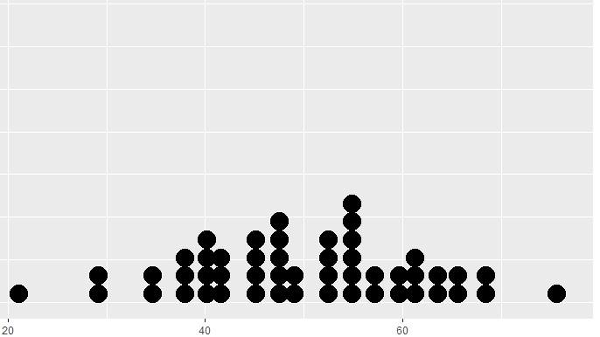Figure 1

x = as.data.frame(rnorm(50,50,10))
ggplot(x, aes(x = x)) + geom_dotplot()

This appears to follow a normal distribution. But how do we get the mean and standard deviation (sd) for this distribution? One way is to directly compute the mean and sd of the given data, which comes out to be 49.8 Kg and 11.37, respectively. These values are a good representation of the given data but may not best describe the population.

We can use MLE in order to get more robust parameter estimates. Thus, MLE can be defined as a method for estimating population parameters (such as the mean and variance for Normal, rate (lambda) for Poisson, etc.) from sample data such that the probability (likelihood) of obtaining the observed data is maximized.

In order to get an intuition of MLE, try to guess which of the following would maximize the probability of observing the data in the above figure.

1. Mean = 100, SD = 10
2. Mean = 50, SD = 10

Clearly, numerically it is not very likely we’ll observe the above data shape if the population mean is 100.

Getting to Know the Technical Details

Now that you got an intuition of what MLE can do, we can get into the details of what the actual likelihood method is and how it can be maximized. But first, let’s start with a quick review of distribution parameters.

Distribution Parameters

Let us first understand distribution parameters. Wikipedia’s definition of this term is as follows: “It is a quantity that indexes a family of probability distributions”. It can be regarded as a numerical characteristic of a population or a statistical model. We can understand it by the following diagram:

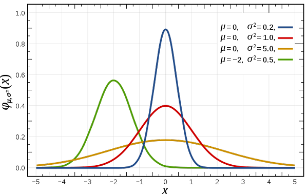Figure 2, Source: Wikipedia

The width and height of the bell curve are conditional and are governed by two parameters – mean and variance. These are known as distribution parameters for normal distribution. Similarly, Poisson distribution is governed by one parameter – lambda, which is the number of times an event occurs in an interval of time or space.

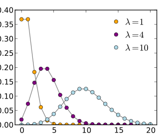Figure 3, Source: Wikipedia

Most of the distributions have one or two parameters, but some distributions can have up to 4 parameters, like a 4 parameter beta distribution.

Likelihood

From Fig. 2 and 3, we can see that given a set of distribution parameters, some data values are more probable than other data. From Fig. 1, we have seen that the given data is more likely to occur when the mean is 50 rather than 100. In reality, however, we have already observed the data. Accordingly, we are faced with an inverse problem: Given the observed data and a model of interest, we need to find the one Probability Density Function/Probability Mass Function (f(x|θ)), among all the probability densities that are most likely to have produced the data.

To solve this inverse problem, we define the likelihood function by reversing the roles of the data vector x and the (distribution) parameter vector θ in f(x| θ), i.e.,

L(θ;x) = f(x| θ)

In MLE, we can assume that we have a likelihood function L(θ;x), where θ is the distribution parameter vector, and x is the set of observations. We are interested in finding the value of θ that maximizes the likelihood with given observations (values of x).

Log Likelihood

The mathematical problem at hand becomes simpler if we assume that the observations (xi) are independent and identically distributed random variables drawn from a Probability Distribution, f0 (where f0 = Normal Distribution, for example, in Fig.1). This reduces the Likelihood function to:

To find the maxima/minima of this function, we can take the derivative of this function w.r.t θ and equate it to 0 (as zero slopes indicate maxima or minima). Since we have terms in product here, we need to apply the chain rule, which is quite cumbersome with products. A clever trick would be to take the log of the likelihood function and maximize the same. This will convert the product to a sum, and since the log is a strictly increasing function, it would not impact the resulting value of θ. So we have:

Maximizing the Likelihood

To find the maxima of the log-likelihood function LL(θ; x), we can:

• Take the first derivative of LL(θ; x) function w.r.t θ and equate it to 0
• Take the second derivative of LL(θ; x) function w.r.t θ and confirm that it is negative

In many situations, calculus is of no direct help in maximizing a likelihood, but a maximum can still be readily identified. There’s nothing that gives setting the first derivative equal to zero any kind of ‘primacy’ or special place in finding the parameter value(s) that maximize log-likelihood. It’s a convenient tool when a few parameters must be estimated.

As a general principle, pretty much any valid approach for identifying the argmax of a function may be suitable to find the maxima of the log-likelihood function. This is an unconstrained non-linear optimization problem. We seek an optimization algorithm that behaves in the following manner:

1. Reliably converge to a local minimizer from an arbitrary starting point
2. Do it as quickly as possible

It’s very common to use optimization techniques to maximize likelihood; there are a large variety of methods (Newton’s method, Fisher scoring, various conjugate gradient-based approaches, steepest descent, Nelder-Mead type (simplex) approaches, BFGS, and a wide variety of other techniques).

It turns out that when the model is assumed to be Gaussian, as in the examples above, the MLE estimates are equivalent to the ordinary least squares method.

You can refer to the proof here.

Determining Model Coefficients Using MLE

Let us now look at how MLE can be used to determine the coefficients of a predictive model.

Suppose that we have a large sample size (asymptotic normality)of n observations y1, y2, . . . , yn which can be treated as realizations of independent Poisson random variables, with Yi ∼ P(µi). Also, suppose that we want to let the mean µi (and therefore the variance!) depend on a vector of explanatory variables xi. We could form a simple linear model as follows:

where θ is the vector of model coefficients. This model has the disadvantage that the linear predictor on the right-hand side can assume any real value, whereas the Poisson mean on the left-hand side, which represents an expected count, has to be non-negative. A straightforward solution to this problem is to model the logarithm of the mean using a linear model. Thus, we consider a generalized linear model with log link log, which can be written as follows:

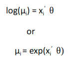
Our aim is to find θ by using MLE.
Now, Poisson distribution is given by:

We can apply the log-likelihood concept that we learned in the previous section to find the θ. Taking logs of the above equation and ignoring a constant involving log(y!), we find that the log-likelihood function is –

where µi depends on the covariates xi and a vector of θ coefficients. We can substitute µi = exp(xi’θ) and solve the equation to get θ that maximizes the likelihood. Once we have the θ vector, we can then predict the expected value of the mean by multiplying the xi and the θ vector.

Maximum Likelihood Estimation Using R

In this section, we will use a real-life dataset to solve a problem using the concepts learned earlier. You can download the dataset from this link.  A sample from the dataset is as follows:

    Date Time Count of tickets sold
25-08-2012 00:00 8
25-08-2012 01:00      2
25-08-2012 02:00      6
25-08-2012 03:00      2
25-08-2012 04:00      2
25-08-2012 05:00      2

It has the count of tickets sold in each hour from 25th Aug 2012 to 25th Sep 2014  (about 18K records). Our aim is to predict the number of tickets sold in each hour. This is the same dataset that was discussed in the first section of this article.

The problem can be solved using techniques like regression, time series, etc. Here we will use the statistical modeling technique that we have learned above using R.

Let’s first analyze the data. In statistical modeling, we are concerned more with how the target variable is distributed. Let’s have a look at the distribution of counts:

hist(Y$Count, breaks = 50,probability = T ,main = "Histogram of Count Variable")
lines(density(Y$Count), col="red", lwd=2)

This could be treated as a Poisson distribution, or we could even try fitting an exponential distribution.

Since the variable at hand is a count of tickets, Poisson is a more suitable model for this. The exponential distribution is generally used to model the time interval between events.

Let’s plot the count of tickets sold over these 2 years:

Looks like there has been a significant increase in the sale of tickets over time. In order to keep things simple, let’s model the outcome by only using age as a factor, where age is the defined no. of weeks elapsed since 25th Aug 2012. We can write this as:

where µ (Count of tickets sold) is assumed to follow the mean of Poisson distribution, and θ0 and θ1 are the coefficients that we need to estimate.

Combining Eq. 1 and 2, we get the log-likelihood function as follows:

We can use the mle() function in R stats4 package to estimate the coefficients θ0 and θ1. It needs the following primary parameters:

1. Negative Likelihood function which needs to be minimized: This is the same as the one that we have just derived, but a negative sign in front [as maximizing the log-likelihood is the same as minimizing the negative log likelihood]
2. Starting point for the coefficient vector: This is the initial guess for the coefficient. Results can vary based on these values as the function can hit local minima. Hence, it’s good to verify the results by running the function with different starting points.
3. Optionally, the method using which the likelihood function should be optimized. BFGS is the default method.

For our example, the negative log-likelihood function can be coded as follows:

nll <- function(theta0,theta1) {
    x <- Y$age[-idx]
    y <- Y$Count[-idx]
    mu = exp(theta0 + x*theta1)
    -sum(y*(log(mu)) - mu)
}

I have divided the data into train and test sets so that we can objectively evaluate the performance of the model. idx is the indices of the rows which are in the test set.

set.seed(200)
idx <- createDataPartition(Y$Count, p=0.25,list=FALSE)

Next, let’s call the mle function to get the parameters:

est <- stats4::mle(minuslog=nll, start=list(theta0=2,theta1=0))
summary(est)

Maximum likelihood estimation
Call:
stats4::mle(minuslogl = nll, start = list(theta0 = 2, theta1 = 0))

Coefficients:
         Estimate  Std. Error
theta0 2.68280754 2.548367e-03
theta1 0.03264451 2.998218e-05

-2 log L: -16594396

This gives us the estimate of the coefficients. Let’s use RMSE as the evaluation metric for getting results on the test set:

pred.ts <- (exp(coef(est)['theta0'] + Y$age[idx]*coef(est)['theta1'] ))
rmse(pred.ts, Y$Count[idx])

86.95227

Now let’s see how our model fairs against the standard linear model (with errors normally distributed), modeled with the log of the count.

lm.fit <-  lm(log(Count)~age, data=Y[-idx,])

Coefficients:
             Estimate Std. Error t value Pr(>|t|)    
(Intercept) 1.9112992 0.0110972   172.2 <2e-16 ***
age         0.0414107 0.0001768   234.3 <2e-16 ***

pred.lm <- predict(lm.fit, Y[idx,])
rmse(exp(pred.lm), Y$Count[idx]) 

93.77393

As you can see, RMSE for the standard linear model is higher than our model with Poisson distribution. Let’s compare the residual plots for these 2 models on a held-out sample to see how the models perform in different regions:

We see that the standard errors using Poisson regression are much closer to zero when compared to Normal linear regression.

A similar thing can be achieved in Python by using the scipy.optimize.minimize() function, which accepts an objective function to minimize, the initial guess for the parameters and methods like BFGS, L-BFGS, etc.

It is further simpler to model popular distributions in R using the glm function from the stats package. It supports Poisson, Gamma, Binomial, Quasi, Inverse Gaussian, Quasi Binomial, and Quasi Poisson distributions out of the box. For the example shown above, you can get the coefficients directly using the below command:

glm(Count ~ age, family = "poisson", data = Y)

Coefficients:
             Estimate Std. Error z value Pr(>|z|)    
(Intercept) 2.669     2.218e-03    1203 <2e-16 ***
age         0.03278   2.612e-05    1255 <2e-16 ***

The same can be done in Python using pymc.glm() and setting the family as pm.glm.families.Poisson().

Conclusion

One way to think of the above example is that there exist random effects or better coefficients in the parameter space than those estimated by a standard linear model. The normal distribution is the default and most widely used form of distribution, but we can obtain better results if the correct distribution is used instead. Maximum likelihood estimation is a technique that can be used to estimate the distribution parameters irrespective of the distribution used. So next time you have a modeling problem at hand, first look at the distribution of data and see if something other than normal makes more sense!

The detailed code and data are present on my Github repository. Refer to the “Modelling single variables.R” file for an example that covers data reading, formatting, and modeling using only age variables. I have also modeled using multiple variables, which is present in the “Modelling multiple variables.R” file.

Key Takeaways

• Maximum likelihood estimation (MLE) is a statistical method that estimates the parameters of a probability distribution based on observed data.
• The goal of MLE is to find the values of parameters that maximize the likelihood function.

Frequently Asked Questions

AanishS Singla 23 May 2023

Aanish is a Data Scientist at Nagarro and has 13+ years of experience in Machine Learning, Developing and Managing IT applications. He is also a volunteer for Delhi chapter of Analytics Vidhya.