Introduction to Monte Carlo Tree Search: The Game-Changing Algorithm behind DeepMind’s AlphaGo
Introduction
A best of five game series, $1 million dollars in prize money – A high stakes shootout. Between 9 and 15 March, 2016, the second-highest ranked Go player, Lee Sidol, took on a computer program named AlphaGo.
AlphaGo emphatically outplayed and outclassed Mr. Sidol and won the series 4-1. Designed by Google’s DeepMind, the program has spawned many other developments in AI, including AlphaGo Zero. These breakthroughs are widely considered as stepping stones towards Artificial General Intelligence (AGI).

In this article, I will introduce you to the algorithm at the heart of AlphaGo – Monte Carlo Tree Search (MCTS). This algorithm has one main purpose – given the state of a game, choose the most promising move.
To give you some context behind AlphaGo, we’ll first briefly look at the history of game playing AI programs. Then, we’ll see the components of AlphaGo, the Game Tree Concept, a few tree search algorithm, and finally dive into how the MCTS algorithm works.
Table of contents
Game AI – A Summary
AI is a vast and complex field. But before AI officially became a recognized body of work, early pioneers in computer science wrote game-playing programs to test whether computers could solve human-intelligence level tasks.

To give you a sense of where Game Playing AI started from and it’s journey till date, I have put together the below key historical developments:
- A. S. Douglas programmed the first software that managed to master a game in 1952. The game? Tic-Tac-Toe! This was part of his doctoral dissertation at Cambridge
- A few years later, Arthur Samuel was the first to use reinforcement learning that to play Checkers by playing against itself
- In 1992, Gerald Tesauro designed a now-popular program called TD-Gammon to play backgammon at a world-class level
- For decades, Chess was seen as “the ultimate challenge of AI”. IBM’s Deep Blue was the first software that exhibited superhuman Chess capability. The system famously defeated Garry Kasparov, the reigning grandmaster of chess, in 1997
- One of the most popular board game AI milestones was reached in 2016 in the game of Go. Lee Sedol, a 9-dan professional Go player, lost a five-game match against Google DeepMind’s AlphaGo software which featured a deep reinforcement learning approach
- Notable recent milestones in video game AI include algorithms developed by Google DeepMind to play several games from the classic Atari 2600 video game console at a super-human skill level
- Last year, OpenAI built the popular OpenAI Five system that mastered the complex strategy game of DOTA
And this is just skimming the surface! There are plenty of other examples where AI programs exceeded expectations. But this should give you a fair idea of where we stand today.
Components of the AlphaGo
The core parts of the Alpha Go comprise of:
- Monte Carlo Tree Search: AI chooses its next move using MCTS
- Residual CNNs (Convolutional Neural Networks): AI assesses new positions using these networks
- Reinforcement learning: Trains the AI by using the current best agent to play against itself
In this blog, we will focus on the working of Monte Carlo Tree Search only. This helps AlphaGo and AlphaGo Zero smartly explore and reach interesting/good states in a finite time period which in turn helps the AI reach human level performance.
It’s application extends beyond games. MCTS can theoretically be applied to any domain that can be described in terms of {state, action} pairs and simulation used to forecast outcomes. Don’t worry if this sounds too complex right now, we’ll break down all these concepts in this article.
The Game Tree Concept
Game Trees are the most well known data structures that can represent a game. This concept is actually pretty straightforward.
Each node of a game tree represents a particular state in a game. On performing a move, one makes a transition from a node to its children. The nomenclature is very similar to decision trees wherein the terminal nodes are called leaf nodes.

For example, in the above tree, each move is equivalent to putting a cross at different positions. This branches into various other states where a zero is put at each position to generate new states. This process goes on until the leaf node is reached where the win-loss result becomes clear.
Tree Search Algorithms
Our primary objective behind designing these algorithms is to find best the path to follow in order to win the game. In other words, look/search for a way of traversing the tree that finds the best nodes to achieve victory.
The majority of AI problems can be cast as search problems, which can be solved by finding the best plan, path, model or function.
Tree search algorithms can be seen as building a search tree:
- The root is the node representing the state where the search starts
- Edges represent actions that the agent takes to go from one state to another
- Nodes represent states
The tree branches out because there are typically several different actions that can be taken in a given state. Tree search algorithms differ depending on which branches are explored and in what order.
Let’s discuss a few tree search algorithms.
Uninformed Search
Uninformed Search algorithms, as the name suggests, search a state space without any further information about the goal. These are considered basic computer science algorithms rather than as a part of AI. Two basic algorithms that fall under this type of search are depth first search (DFS) and breadth first search (BFS). You can read more about them in this blog post.

Best First Search
The Best First Search (BFS) method explores a graph by expanding the most promising node chosen according to a specific rule. The defining characteristic of this search is that, unlike DFS or BFS (which blindly examine/expand a cell without knowing anything about it), BFS uses an evaluation function (sometimes called a “heuristic”) to determine which node is the most promising, and then examines this node.
For example, A* algorithm keeps a list of “open” nodes which are next to an explored node. Note that these open nodes have not been explored. For each open node, an estimate of its distance from the goal is made. New nodes are chosen to explore based on the lowest cost basis, where the cost is the distance from the origin node plus the estimate of the distance to the goal.
Minimax
For single-player games, simple uninformed or informed search algorithms can be used to find a path to the optimal game state. What should we do for two-player adversarial games where there is another player to account for? The actions of both players depend on each other.
For these games, we rely on adversarial search. This includes the actions of two (or more) adversarial players. The basic adversarial search algorithm is called Minimax.
This algorithm has been used very successfully for playing classic perfect-information two-player board games such as Checkers and Chess. In fact, it was (re)invented specifically for the purpose of building a chess-playing program.
The core loop of the Minimax algorithm alternates between player 1 and player 2, quite like the white and black players in chess. These are called the min player and the max player. All possible moves are explored for each player.
For each resulting state, all possible moves by the other player are also explored. This goes on until all possible move combinations have been tried out to the point where the game ends (with a win, loss or draw). The entire game tree is generated through this process, from the root node down to the leaves:

Each node is explored to find the moves that give us the maximum value or score.
What are the reasons for employing Monte Carlo Tree Search (MCTS)?
Smart Decision-Making:
MCTS is a clever algorithm for making decisions in complex situations, like games, where there are many choices.
Learns as It Goes:
Even with incomplete information, MCTS can learn and improve over time, adapting to different scenarios.
Step-by-Step Choices:
It’s effective for making decisions one after another, especially in situations where choices affect each other.
Balanced Exploration:
MCTS strikes a balance between trying out new possibilities and using what it already knows to make informed decisions.
Versatile Applications:
Beyond games, MCTS can be applied to various problems, offering solutions for decision-making in different domains.
Monte Carlo Tree Search
Games like tic-tac-toe, checkers and chess can arguably be solved using the minimax algorithm. However, things can get a little tricky when there are a large number of potential actions to be taken at each state. This is because minimax explores all the nodes available. It can become frighteningly difficult to solve a complex game like Go in a finite amount of time.
Go has a branching factor of approximately 300 i.e. from each state there are around 300 actions possible, whereas chess typically has around 30 actions to choose from. Further, the positional nature of Go, which is all about surrounding the adversary, makes it very hard to correctly estimate the value of a given board state. For more information on rules for Go, please refer this link.

There are several other games with complex rules that minimax is ill-equipped to solve. These include Battleship Poker with imperfect information and non-deterministic games such as Backgammon and Monopoly. Monte Carlo Tree Search, invented in 2007, provides a possible solution.
The basic MCTS algorithm is simple: a search tree is built, node-by-node, according to the outcomes of simulated playouts. The process can be broken down into the following steps:
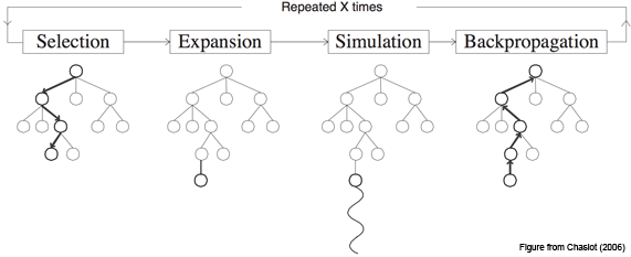
- Selection
Selecting good child nodes, starting from the root node R, that represent states leading to better overall outcome (win). - Expansion
If L is a not a terminal node (i.e. it does not end the game), then create one or more child nodes and select one (C). - Simulation (rollout)
Run a simulated playout from C until a result is achieved. - Backpropagation
Update the current move sequence with the simulation result.
Tree Traversal & Node Expansion
Before we delve deeper and understand tree traversal and node expansion, let’s get familiar with a few terms.
UCB Value
UCB1, or upper confidence bound for a node, is given by the following formula:

where,
- Vi is the average reward/value of all nodes beneath this node
- N is the number of times the parent node has been visited, and
- ni is the number of times the child node i has been visited
Rollout
What do we mean by a rollout? Until we reach the leaf node, we randomly choose an action at each step and simulate this action to receive an average reward when the game is over.
Loop Forever:

if Si is a terminal state:

   return Value(Si)

Ai = random(available_actions(Si))

Si = Simulate(Si, Ai)

This loop will run forever until you reach a terminal state.

Tree Traversal & Node Expansion
You start with S0, which is the initial state. If the current node is not a leaf node, we calculate the values for UCB1 and choose the node that maximises the UCB value. We keep doing this until we reach the leaf node.
Next, we ask how many times this leaf node was sampled. If it’s never been sampled before, we simply do a rollout (instead of expanding). However, if it has been sampled before, then we add a new node (state) to the tree for each available action (which we are calling expansion here).
Your current node is now this newly created node. We then do a rollout from this step.
Complete Walkthrough with an example
Let’s do a complete walkthrough of the algorithm to truly ingrain this concept and understand it in a lucid manner.
Iteration 1:
- We start with an initial state S0. Here, we have actions a1 and a2 which lead to states s1 and s2 with total score t and number of visits n. But how do we choose between the 2 child nodes?

- This is where we calculate the UCB values for both the child nodes and take whichever node maximises that value. Since none of the nodes have been visited yet, the second term is infinite for both. Hence, we are just going to take the first node
- We are now at a leaf node where we need to check whether we have visited it. As it turns out, we haven’t. In this case, on the basis of the algorithm, we do a rollout all the way down to the terminal state. Let’s say the value of this rollout is 20

- Now comes the 4th phase, or the backpropogation phase. The value of the leaf node (20) is backpropogated all the way to the root node. So now, t = 20 and n = 1 for nodes S1 and S0

- That’s the end of the first iteration
The way MCTS works is that we run it for a defined number of iterations or until we are out of time. This will tell us what is the best action at each step that one should take to get the maximum return.
Iteration 2:
- We go back to the initial state and ask which child node to visit next. Once again, we calculate the UCB values, which will be 20 + 2 * sqrt(ln(1)/1) = 20 for S1 and infinity for S2. Since S2 has the higher value, we will choose that node
- Rollout will be done at S2 to get to the value 10 which will be backpropogated to the root node. The value at root node now is 30

Iteration 3:
- In the below diagram, S1 has a higher UCB1 value and hence the expansion should be done here:

- Now at S1, we are in exactly the same position as the initial state with the UCB1 values for both nodes as infinite. We do a rollout from S3 and end up getting a value of 0 at the leaf node
Iteration 4:
- We again have to choose between S1 and S2. The UCB value for S1 comes out to be 11.48 and 12.10 for S2:

- We’ll do the expansion step at S2 since that’s our new current node. On expansion, 2 new nodes are created – S5 and S6. Since these are 2 new states, a rollout is done till the leaf node to get the value and backpropogate
That is the gist of this algorithm. We can perform more iterations as long as required (or is computationally possible). The underlying idea is that the estimate of values at each node becomes more accurate as the number of iterations keep increasing.
Conclusion
Deepmind’s AlphaGo and AlphaGo Zero programs are far more complex with various other facets that are outside the scope of this article. However, the Monte Carlo Tree Search algorithm remains at the heart of it. MCTS plays the primary role in making complex games like Go easier to crack in a finite amount of time. Some open source implementations of MCTS are linked below:
I expect reinforcement learning to make a lot of headway in 2019. It won’t be surprising to see a lot more complex games being cracked by machines soon. This is a great time to learn reinforcement learning!
I would love to hear your thoughts and suggestions regarding this article and this algorithm in the comments section below. Have you used this algorithm before? If not, which game would you want to try it out on?
Frequently Asked Questions
MCTS is like a clever way of making decisions, especially in complicated situations. It’s like trying different things randomly and learning from them to determine the best choices.
a. Adapts Well: MCTS is good at handling situations where we don’t know everything.
b. Balances Trying New and Known Things: It’s like being good at trying new ideas and using what you already know.
c. Works in Different Situations: MCTS isn’t just for games; it can help with all sorts of problems.
d. Good for Step-by-Step Decisions: It’s great for situations where you must make decisions one after another.
e. Does Well in Games: MCTS is like a friend who’s good at playing games like chess and Go.
a. Needs a Lot of Computer Power: MCTS can be demanding on computers, especially in situations with many choices.
b. Can Be a Bit Random: Depending on luck, too much might mean it only sometimes makes the absolute best decisions.
c. Tricky to Set Up Just Right: It’s like adjusting settings; getting them right can be tricky.
d. Might Miss Some Good Choices: Sometimes, it only sees some of the best options and could miss out on great moves.
e. Learns from Limited Info: Learning from just some information might only sometimes lead to the smartest decisions.
IIT Bombay Graduate with a Masters and Bachelors in Electrical Engineering. I have previously worked as a lead decision scientist for Indian National Congress deploying statistical models (Segmentation, K-Nearest Neighbours) to help party leadership/Team make data-driven decisions. My interest lies in putting data in heart of business for data-driven decision making.


Is it Best First Search Tree or Breadth First Search Tree?
Hi Vamsi, this is best first search as this is not uninformed tree search. For more information go to this link: https://en.wikipedia.org/wiki/Best-first_search
Thank you . It was easy to understand .
Great article, brilliant explanation!