6 Powerful Feature Engineering Techniques For Time Series Data (using Python)
Overview
- Feature engineering is a skill every data scientist should know how to perform, especially in the case of time series
- We’ll discuss 6 powerful feature engineering techniques for time series in this article
- Each feature engineering technique is detailed using Python
Introduction
‘Time’ is the most essential concept in any business. We map our sales numbers, revenue, bottom line, growth, and even prepare forecasts – all based on the time component.
But consequently, this can be a complex topic to understand for beginners. There is a lot of nuance to time series data that we need to consider when we’re working with datasets that are time-sensitive.
Existing time series forecasting models undoubtedly work well in most cases, but they do have certain limitations. I’ve seen aspiring data scientists struggle to map their data when they’re given only the time component and the target variable. It’s a tricky challenge but not an impossible one.

There’s no one-size-fits-all approach here. We don’t have to force-fit traditional time series techniques like ARIMA all the time (I speak from experience!). There’ll be projects, such as demand forecasting or click prediction when you would need to rely on supervised learning algorithms.
And there’s where feature engineering for time series comes to the fore. This has the potential to transform your time series model from just a good one to a powerful forecasting model.
In this article, we will look at various feature engineering techniques for extracting useful information using the date-time column. And if you’re new to time series, I encourage you to check out the below free course:
Table of contents
- Overview
- Introduction
- Quick Introduction to Time Series
- Setting up the Problem Statement for Time Series Data
- Feature Engineering for Time Series #1: Date-Related Features
- Feature Engineering for Time Series #2: Time-Based Features
- Feature Engineering for Time Series #3: Lag Features
- Feature Engineering for Time Series #4: Rolling Window Feature
- Feature Engineering for Time Series #5: Expanding Window Feature
- Feature Engineering for Time Series #6: Domain-Specific Features
- Validation Technique for Time Series
- Frequently Asked Questions
- End Notes
Quick Introduction to Time Series
Before we look at the feature engineering techniques, let’s brush over some basic time series concepts. We’ll be using them throughout the article so it’s best to be acquainted with them here.
So, what makes time series projects different from the traditional machine learning problems?
In a time series, the data is captured at equal intervals and each successive data point in the series depends on its past values.
Let’s take a simple example to understand this. If we want to predict today’s stock price for a certain company, it would be helpful to have information about yesterday’s closing price, right? Similarly, predicting the traffic on a website would be a lot easier if we have data about the last few months or years.
There’s another thing we need to consider – time series data may also have certain trends or seasonality. Take a look at the plot shown below about the number of tickets booked for an airline over the years:
We can clearly see an increasing trend. Such information can be useful for making more accurate predictions. Now, let’s take a dataset with date-time variables and start learning about feature engineering!
Setting up the Problem Statement for Time Series Data
We’ll be working on a fascinating problem to learn feature engineering techniques for time series.
We have the historical data for ‘JetRail’, a form of public rail transport, that uses advanced technology to run rails at a high speed. JetRail’s usage has increased recently and we have to forecast the traffic on JetRail for the next 7 months based on past data.
Let’s see how we can help JetRail’s management team solve this problem. You can go through the detailed problem statement and download the dataset from here.
Let’s load the dataset in our notebook:
We have two columns here – so it’s clearly a univariate time series. Also, the data type of the date variable is taken as an object, i.e. it is being treated as a categorical variable. Hence, we will need to convert this into a DateTime variable. We can do this using the appropriately titled datetime function in Pandas:
Now that we have the data ready, let’s look at the different features we can engineer from this variable. Along with each of these feature engineering techniques, we will discuss different scenarios where that particular technique can be useful.
NOTE: I have taken a simple time series problem to demonstrate the different feature engineering techniques in this article. You can use them on a dataset of your choice as long as the date-time column is present.
Feature Engineering for Time Series #1: Date-Related Features
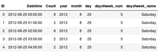
Have you ever worked in a product company? You’ll be intimately familiar with the task of forecasting the sales for a particular product. We can find out the sales pattern for weekdays and weekends based on historical data. Thus, having information about the day, month, year, etc. can be useful for forecasting the values.
Let’s get back to our JetRail project.
We have to forecast the count of people who will take the JetRail on an hourly basis for the next 7 months. This number could be higher for weekdays and lower for weekends or during the festive seasons. Hence, the day of the week (weekday or weekend) or month will be an important factor.
Extracting these features is really easy in Python:
Feature Engineering for Time Series #2: Time-Based Features
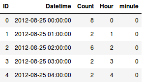
We can similarly extract more granular features if we have the time stamp. For instance, we can determine the hour or minute of the day when the data was recorded and compare the trends between the business hours and non-business hours.
If we are able to extract the ‘hour’ feature from the time stamp, we can make more insightful conclusions about the data. We could find out if the traffic on JetRail is higher during the morning, afternoon or evening time. Or we could use the value to determine the average hourly traffic throughout the week, i.e. the number of people who used JetRail between 9-10 am, 10-11 am, and so on (throughout the week).
Extracting time-based features is very similar to what we did above when extracting date-related features. We start by converting the column to DateTime format and use the .dt accessor. Here’s how to do it in Python:
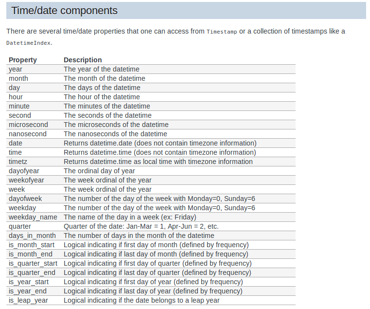
Similarly, we can extract a number of features from the date column. Here’s a complete list of features that we can generate:
Run the code below to generate the date and hour features for the given data. You can select any of the above functions and run the following code to generate a new feature for the same!
Feature Engineering for Time Series #3: Lag Features
Here’s something most aspiring data scientists don’t think about when working on a time series problem – we can also use the target variable for feature engineering!
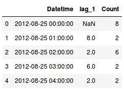
Consider this – you are predicting the stock price for a company. So, the previous day’s stock price is important to make a prediction, right? In other words, the value at time t is greatly affected by the value at time t-1. The past values are known as lags, so t-1 is lag 1, t-2 is lag 2, and so on.
Here, we were able to generate lag one feature for our series. But why lag one? Why not five or seven? That’s a good question.
The lag value we choose will depend on the correlation of individual values with its past values.
If the series has a weekly trend, which means the value last Monday can be used to predict the value for this Monday, you should create lag features for seven days. Getting the drift?
We can create multiple lag features as well! Let’s say we want lag 1 to lag 7 – we can let the model decide which is the most valuable one. So, if we train a linear regression model, it will assign appropriate weights (or coefficients) to the lag features:
There is more than one way of determining the lag at which the correlation is significant. For instance, we can use the ACF (Autocorrelation Function) and PACF (Partial Autocorrelation Function) plots.
- ACF: The ACF plot is a measure of the correlation between the time series and the lagged version of itself
- PACF: The PACF plot is a measure of the correlation between the time series with a lagged version of itself but after eliminating the variations already explained by the intervening comparisons
For our particular example, here are the ACF and PACF plots:
from statsmodels.graphics.tsaplots import plot_acf
plot_acf(data['Count'], lags=10)
plot_pacf(data['Count'], lags=10)
The partial autocorrelation function shows a high correlation with the first lag and lesser correlation with the second and third lag. The autocorrelation function shows a slow decay, which means that the future values have a very high correlation with its past values.
An important point to note – the number of times you shift, the same number of values will be reduced from the data. You would see some rows with NaNs at the start. That’s because the first observation has no lag. You’ll need to discard these rows from the training data.
Feature Engineering for Time Series #4: Rolling Window Feature
In the last section, we looked at how we can use the previous values as features.
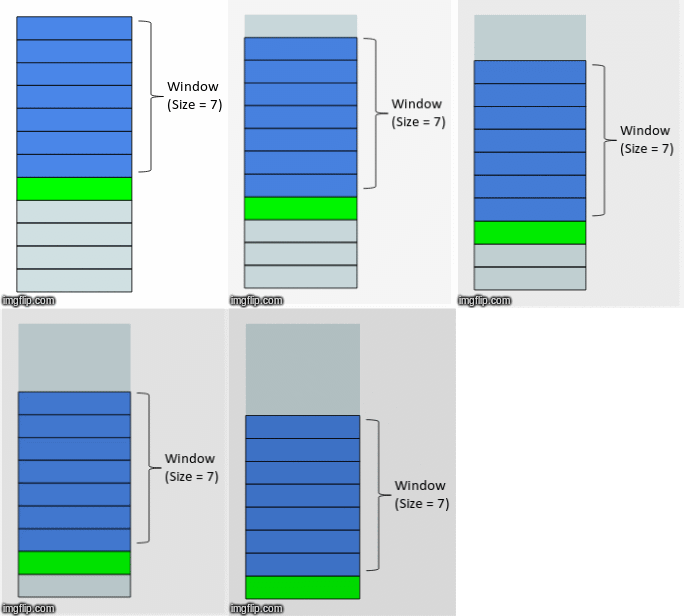
How about calculating some statistical values based on past values? This method is called the rolling window method because the window would be different for every data point.
Here’s an awesome gif that explains this idea in a wonderfully intuitive way:
Since this looks like a window that is sliding with every next point, the features generated using this method are called the ‘rolling window’ features.
Now the question we need to address – how are we going to perform feature engineering here? Let’s start simple. We will select a window size, take the average of the values in the window, and use it as a feature. Let’s implement it in Python:
Similarly, you can consider the sum, min, max value, etc. (for the selected window) as a feature and try it out on your own machine.
Recency in an important factor in a time series. Values closer to the current date would hold more information.
Thus, we can use a weighted average, such that higher weights are given to the most recent observations. Mathematically, weighted average at time t for the past 7 values would be:
w_avg = w1*(t-1) + w2*(t-2) + . . . . + w7*(t-7)
where, w1>w2>w3> . . . . >w7.
Feature Engineering for Time Series #5: Expanding Window Feature
This is simply an advanced version of the rolling window technique. In the case of a rolling window, the size of the window is constant while the window slides as we move forward in time. Hence, we consider only the most recent values and ignore the past values.
The idea behind the expanding window feature is that it takes all the past values into account.
Here’s a gif that explains how our expanding window function works:
As you can see, with every step, the size of the window increases by one as it takes into account every new value in the series. This can be implemented easily in Python by using the expanding() function. Let’s code this using the same data:
Here is a live coding window that generates the expanding window feature for the given data. Feel free to change the starting window size and print the results:
Feature Engineering for Time Series #6: Domain-Specific Features
This is the essence of feature engineering!
Having a good understanding of the problem statement, clarity of the end objective and knowledge of the available data is essential to engineer domain-specific features for the model.
Want to dive into this more? Let’s take an example.
Below is the data provided by a retailer for a number of stores and products. Our task is to forecast the future demands for the products. We can come up with various features, like taking a lag or averaging the past values, among other things.
But hold on. Let me ask you a question – would it be the right way to build lag features from lag(1) to lag(7) throughout the data?
Certainly not! There are different stores and products, and the demand for each store and product would be significantly different. In this case, we can create lag features considering the store-product combination. Moreover, if we have knowledge about the products and the trends in the market, we would be able to generate more accurate (and fewer) features.
Not only this, having a good understanding about the domain and data would help us in selecting the lag value and the window size. Additionally, based on your domain knowledge, you would be able to pull external data that adds more value to the model.
Here’s what I mean – are the sales affected by the weather on the day? Will the sales increase/decrease on a national holiday? If yes, then you can use external datasets and include the list of holidays as a feature.
Validation Technique for Time Series
All the feature engineering techniques we have discussed can be used to convert a time series problem into a supervised machine learning problem.
Once we have that, we can easily go ahead with machine learning algorithms like linear regression and random forest. But there is one important step that you should know before you jump to the model building process – creating a validation set for time series.
For the traditional machine learning problems, we randomly select subsets of data for the validation and test sets. But in these cases, each data point is dependent on its past values. If we randomly shuffle the data, we might be training on future data and predicting the past values!
It is important that we carefully build a validation set when working on a time series problem, without destroying the sequential order within the data.
Let’s create a validation set for our problem. But first, we must check the duration for which we have the data:
import pandas as pd
data = pd.read_csv('Train_SU63ISt.csv')
data['Datetime'] = pd.to_datetime(data['Datetime'],format='%d-%m-%Y %H:%M')
data['Datetime'].min(), data['Datetime'].max(), (data['Datetime'].max() -data['Datetime'].min())
(Timestamp('2012-08-25 00:00:00'),
 Timestamp('2014-09-25 23:00:00'),
 Timedelta('761 days 23:00:00'))
We have data for almost 25 months. Let’s save three months for validation and use the remaining for training:
data.index = data.Datetime
Train=data.loc['2012-08-25':'2014-06-24']
valid=data.loc['2014-06-25':'2014-09-25']

Train.shape, valid.shape
((16056, 3), (2232, 3))
Great! We have the train and validation sets ready. You can now use these feature engineering techniques and build machine learning models on this data!
Frequently Asked Questions
A. The features of a time series are the characteristics and patterns observed within the data over time. Some of the key features include:
1. Trend: The long-term movement or direction in the data, indicating overall growth or decline.
2. Seasonality: Regular and predictable patterns that repeat at fixed intervals.
3. Cyclic Patterns: Longer-term oscillations with varying periods, not necessarily repeating at fixed intervals.
4. Noise: Random fluctuations or irregularities in the data that do not follow any specific pattern.
5. Autocorrelation: The correlation of a time series with its own past values at different lags.
6. Level: The baseline or starting point of the time series data.
Understanding these features is essential for time series analysis and forecasting.
A. Time series feature extraction methods involve transforming raw time series data into a set of relevant and informative features. Techniques like moving averages, exponential smoothing, Fourier transforms, wavelet transforms, and statistical measures (mean, variance, etc.) are used to extract characteristics such as trend, seasonality, periodicity, and statistical properties. These features are then used for time series analysis, classification, and forecasting tasks.
End Notes
Time Series is often considered a difficult topic to master. That’s understandable because there are a lot of moving parts when we’re working with the date and time components. But once you have a hang of the basic concepts and are able to perform feature engineering, you’ll be gliding through your projects in no time.
In this article, we discussed some simple techniques that you can use to work with time series data. Using these feature engineering techniques, we can convert any time series problem into a supervised learning problem and build regression models.
Have any questions? Or want to share any other feature engineering techniques for time series? Let’s discuss in the comments section below.
And if you’re new to the world of time series, here is an excellent (and free) course to get you started: Creating Time Series Forecast using Python.





Thanks for this post. That helps I am confused with this command ' data['rolling_mean'] = data['Count'].rolling(window=7).mean()'. I try this command but the output is different from yours. It seems to me your one is window=3, but if window=3, the Rolling mean is NaN,NaN,5.33,3.33,3.33,etc. The first two rollling mean should be NaN which matches yours but the rolling means after the first two are very different from yours. Will u please double check your dataset? I find the dataset here. https://github.com/agarwalpooja/time_series_analysis/find/master?q= Please advise
Hi Aishwarya, I am fresher in machine learning and deep learning. I am currently working on a project of sales prediction. I was wondering if sales prediction is possible other than straight line forecasting which we did using fbprophet which is typically using time series forecasting in the background. We were considering doing this for restaurants and can we have a model based on various attributes affecting a restaurant? If so, what would be the apt machine learning or deep learning method for predicting a useful outcome?
It was helpful. thanks. I want to draw your attention to following point: lag means the previous time-step, not value maybe you can say time-value. that can be confusing!
Hi Aishwarya, My question may not be really related to this ,but for one of your old article on stock price prediction using machine learning (linear regression ,lstm etc.).I could not comment for that post as its moderated . Coming to the question, while using linear regression ,lstm models to predict the prices we pass the test data to predict function (closing_price = model.predict(X_test)) ,where X_test is already a part of the available data set. How can we use this to predict the future prices ? As predict() needs a argument to be passed and the model predicts according to values of X_test(arguments). I used the complete data set to train the model but now stuck while passing the X_test . I used last few rows train data as X_test but the result turned out to be satisfying to the set of train data which I passed to X_test but not to the Valid_data(the data set used to verify the model). When I was going through the comments I found your comment stated below but could not follow it : "Hi Ravi, I actually did finally train my model on the complete data and predicted for next 10 days (and checked against the results for the week). The first 2 predictions weren’t exactly good but next 3 were (didn’t check the remaining). Secondly, I agree that machine learning models aren’t the only thing one can trust, years of experience & awareness about what’s happening in the market can beat any ml/dl model when it comes to stock predictions. I wanted to explore this domain and I have learnt more while working on this dataset than I did while writing my previous articles." can you please let me know how was it done for the next 10 days? One more question I got which is, In what way does these model make sense as we pass the actual data(argument )to predict the model i.e. the resulting predictions will be based on argument passed (X_test) instead of predicting future data as ARIMA model does using the train data. or how can these models used to predict the upcoming data? can you please help me on this? Thanks, Sharan