Game Theory 101: Decision Making in a Competitive Scenario using Normal Form Games
Overview
- Game Theory can be incredibly helpful for decision making in competitive scenarios
- Understand the concept of Normal Form Games in the context of Game Theory
- We’ll also cover the applications of Game Theory with real-world examples
Introduction
Let’s start this article on Game Theory with an example of a game (I love the symbolism!). Football is the most popular sport in the world so we’ll consider a scenario from there.
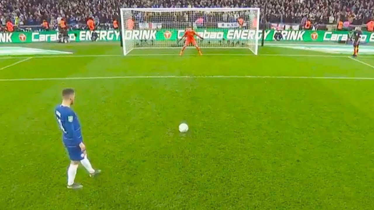
Consider that a team has been awarded a penalty kick. This situation pits the striker against the goalkeeper in a battle of wits. The goalkeeper has to take a decision on whether to leap to the left or the right (or stand his ground). The striker has a similar dilemma (which direction to choose).
Now here’s a question for you – what would you do? If this penalty kick exercise is repeated 10 times, which side would you save as the goalkeeper to minimize the goals scored? Or where would you strike to maximize your goals scored? What action will you take if you have inferences from the past about the performance of the kicker and goalie?
That’s a tough decision. This is where we can apply Game Theory and draw a logical conclusion which suits individual interests:
- Game Theory will take all the big data into consideration while processing the decision
- It will share the rationale behind the decision it suggests, so you know how it arrived at that decision
- The teams will know why and how that decision was taken by using Game Theory
This strategic decision making is an intelligent move from a business perspective considering the fact that the most likely outcomes can be predicted using the inferences and Game Theory.
In this article, we will be primarily looking at Normal Form Games or Simultaneous Games and calculating the Nash Equilibria for the respective games. We will also learn how to compute Nash Equilibrium in Pure Strategy and the Mixed Strategy Games. Finally, we will find the Nash Equilibrium strategy in the penalty kick example above.
I would suggest reading the first article on Game Theory before progressing ahead. That will give you a bird’s eye view of Game Theory and an understanding of how Game Theory is being used in the field of Artificial Intelligence.
Table of Contents
- What Is Game Theory?
- Game Theory – Setting the Stage for Normal Form Games
- Pure Strategy Nash Equilibrium
- Mixed Strategy Nash Equilibria
- Deriving a Solution Using Game Theory
- How is Game Theory Useful for Data Science Professionals?
What Is Game-Theory?
In simple terms – Game Theory happens to be a very specialized subject for any given data Scientist. It allows decision making based on the inferences from the data in the most optimal way possible based on the inferences made after undertaking Big Data Analytics.
Strategic decision making is an intelligent move from a business perspective considering the fact that the most likely outcomes can be predicted using the inferences and Game Theory.
Game Theory helps in predicting how rational people will make decisions that help data scientists make effective data-driven decisions under strategic circumstances. You can ready about this in much more detail here.
Game Theory – Setting the Stage for Normal Form Games
Before we dive into the concept of Normal Form Games, please revise the key terms of Game Theory that we covered in the introductory article.
For your reference, I’ll quickly revise those terms below:
- Game: In a general sense, a game comprises a set of players, actions/strategies and the final payoff. Example: Auction, Chess, Politics, etc.
- Players/Agents: Players are rational entities that participate in any game. For example:
- Bidders in an auction setting
- Politicians participating in elections, etc.
- Actions: They are a set of actions that each agent can take in a game. One thing to note – the actions to any agent may be similar or different depending upon the game
- Game Matrix: It is a systematic representation of all the possible outcomes and rewards based on what action each agent chose. We will be looking at this soon
- Rewards/Payoff: This is simply the reward that any agent receives when an outcome is achieved due to the combined actions of all the agents
Now that we have an idea about the fundamental terms in Game Theory, let’s discuss some of the assumptions that we will be following in this article to understand normal form games.
Assumption 1: Games of Perfect Information
In the context of Game Theory, we have to pay special attention to the amount of information every agent has. There are scenarios where the agents do not know anything about each other. And on the other hand, there are scenarios where agents know everything about each other.
As we are just starting out in Game Theory, we will be dealing with the games of Perfect Information (the latter scenario).
In a perfect information setting, every agent has information about the following:
- All the set of actions that other agents can take
- About the motivation of the other agent
- Knowledge about all the possible outcomes
- Reward the other agents for each outcome possible
- What actions the other agents are taking
- All the agents are rational
Or in essence:
But there are also games of imperfect and incomplete information. However, we will be focusing on them in future articles.
Assumption 2: Simultaneous Actions
In normal form games, we assume that all the agents are taking action simultaneously and they cannot see beforehand what the other agent is going to play.
However, there are scenarios where the agents play a turn-based game – these are known as Extensive Form Games. We will be exploring these forms of games in my next article.
Understanding Normal Form Games
I am assuming that you are already familiar with the Game Matrix that we use in Normal Form Games. In the previous article, we covered the example of a prisoner’s dilemma in detail. It looked something like this:
Now, the easiest thing to start with would be to use this game matrix and learn how this Game is defined. Remember – a Game is defined as a tuple {Players, Actions, Utility}.
Let’s see what each of these represent corresponding to this game matrix above.
Players:
This is the number of players participating in any game. In this Game: Players = {Alan, Ben}.
Actions:
Actions represent the set of actions each agent can take. We should keep in mind that not all players can take all actions. In this Game:
- Actions of Ben = {Confess, Silent}
- Actions of Alan = {Confess, Silent}
Utility/Reward:
The utility or reward of each player is the reward each agent gets corresponding to the actions played by both of them. It is defined using a function of their Actions.
If we represent the actions of Alan as {Aconfess, Asilent} and Ben’s actions as {Bconfess, Bsilent}, then the utility function can be defined as:
- Aconfess , Bconfess = {-10,-10}
- Aconfess , Bsilent = {0,-15}
- Asilent , Bconfess = {-15,0}
- Asilent , Bsilent = {-1,-1}
To understand this notation, let’s break down the third utility function. It says that when Alan stays silent and Ben confesses, they get a utility/reward of -15 and 0 respectively.
And that is Normal Form Games!
Now that we have established an understanding of a normal form game, here is another game matrix:
Before we move on, there’s something I want you to do. Go ahead and try to define the Game{Players, Actions, Utility} for this Game matrix. It will really help you ingrain the concepts we covered in this section. Post your answer in the comments section below!
Pure Strategy Nash Equilibrium
Now that we have understood the nuances of normal form games, let’s look at how to find the Nash Equilibria for these games. You should be familiar with what Nash Equilibria means if you’ve gone through the previous article. Don’t worry if you haven’t, I will cover it briefly here.
Nash Equilibria is defined as the strategy for each agent such that, that strategy is the best response to all the other agents.
Or,
Nash equilibrium is a set of strategies played by each agent such that no one would want to deviate or change their strategy.
In Pure Strategy Nash Equilibrium, the pure stands for a single action which is the best response to all the other agents. Moreover, this pure strategy equilibrium is often referred to as the dominating strategy.
Please pay special attention to the two words – dominating and dominated. They sound very similar and can cause confusion. We will be using both of these words soon so just keep this in mind.
Iterated Removal of Dominated Strategy (IRDS)
To find the Nash Equilibrium in pure strategy, we follow a method known as “Iterated Removal of Dominated Strategy (IRDS)”. This is a simple method that says we can remove the dominated action from the player’s actions if it is clearly dominated by some other better action.
Let’s get back to the example of the Prisoner’s dilemma and workout this strategy:
 Let’s apply the IRDS to Alan’s actions first:
For Alan, there are two possibilities depending upon what Ben does:
- If Ben chooses to confess, it is rational for Alan to confess because 10 years of punishment is better than 15 years of punishment
- If Ben chooses to stay silent, it is rational for Alan to confess because no punishment is better than 1 year of punishment
As a result, no matter what Ben chooses, confessing is a dominating strategy for Alan. Or, deviating from a confession will incur more punishment for Alan. Therefore, we eliminate the dominated action (silent row for Alan is Greyed out).
Now let’s apply the IRDS to Ben’s Actions. There are two possibilities depending upon what Alan does:
- If Alan chooses to confess, it is rational for Ben to confess because 10 years of punishment is better than 15 years of punishment
- If Alan chooses to stay silent, it is rational for Ben to confess because no punishment is better than 1 year of punishment
And we can clearly observe that after the removal of the purely dominated strategy, we are left with the Nash equilibrium {confess, confess} in the prisoner’s dilemma and the resultant utility is {-10,-10}.
I would like you to try out the IRDS method on the following game matrix to practice yourself:
Issues with Pure Strategy Nash Equilibria
Often the games we encounter for decision making are not so simple and may not have a dominant strategy within them. A popular example of one such game is “Matching Pennies”.
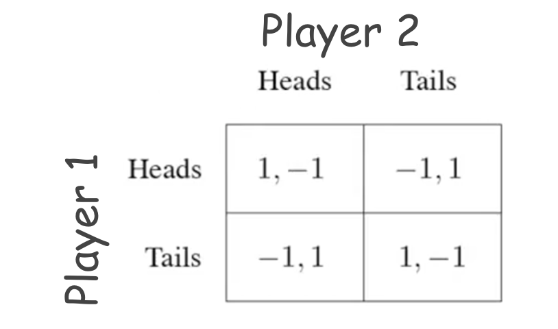
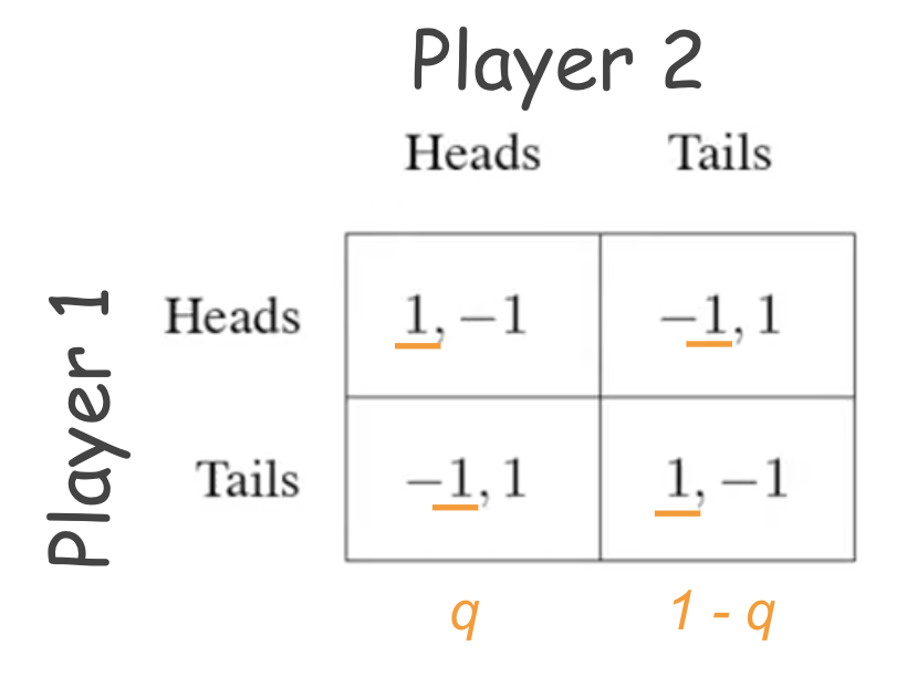
This is a competitive game where the two players have contradicting objectives. The two players have to place a coin over a table and choose which side of the coin should face up. Player 1’s objective is to match the other player’s coin, whereas player 2’s objective is to mismatch with the other player’s coin. The resultant game matrix looks like this:
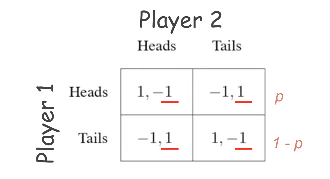
Now, if we take a closer look at this game, applying IRDS is not feasible. For any given actions set from the two players, one of them will always have an incentive to deviate from the current action:
We can clearly see that playing a pure action strategy is a bad idea. As a result, there is no pure-strategy Nash equilibrium. So what do we do?
Mixed Strategy Nash Equilibria
We are going to mix things up! We are going to play some combination of available actions for any agent. Now, it is a no brainer that we cannot play half Heads or half Tails in a single game.
Therefore, we will take the help of probability to mix the action strategies when the games are played repeatedly.
Now, before we jump into mixed strategy and calculate the mixed strategy Nash equilibria, let’s first clear some assumptions of probability:
- Probability of all actions must be non-negative: This means that any action available to any given player should be a number between 0 or 1 (it cannot be greater than 1 or less than 0)
- Total probability = 1: Probabilities of all the actions for any player must sum up to the value of 1
So, how does the mixed strategy work?
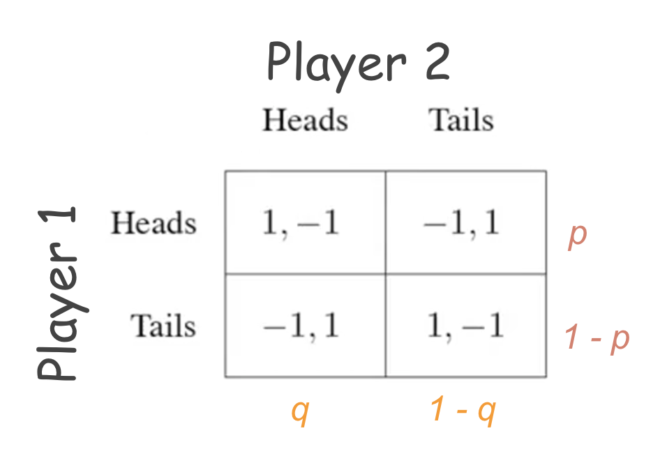
We simply distribute the probability between the actions available to the agents. Consider the matching pennies example above. Player 1 plays “heads” with probability p and plays “tails” with probability “1-p”. Similarly, Player 2 plays “heads” and “tails” with probability q and 1-q.
When players use this mixed strategy, the other players simply cannot stick to a simple or pure action strategy. Hence, they will also need to play in a similar fashion. But the question stays – how do we find the Nash Equilibrium?
To answer this, we will need to understand two things:
- How to calculate utility/reward in mind strategy games
- Exploit the definition of Nash equilibrium
Let’s understand each of these in a bit more detail.
How to calculate utility/reward in mixed strategy games
We calculate the Expected reward/utility when it comes to mixed strategy games. As we are dealing with probabilities, we need to consider them for calculating the expected utility:
The expected payoff for each player “i” in any normal form game is given as:
Sum over all possible outcomes k (reward of getting an outcome k * joint probability of that outcome k being played by all players).
Let’s look at an example:
For player 1:
- Expected payoff from the first outcome: (p)*(q)*(1)
- Expected payoff from the second outcome: (p)*(1 – q)*(-1)
- Expected payoff from the third outcome: (1 – p)*(q)*(-1)
- Expected payoff from the fourth outcome: (1 – p)*(1 – q)*(1)
Total expected payoff for player 1 = sum over all the above outcomes.
Similarly for player 2:
- Expected payoff from first outcome: (p)*(q)*(-1)
- Expected payoff from the second outcome: (p)*(1 – q)*(1)
- Expected payoff from the third outcome: (1 – p)*(q)*(1)
- Expected payoff from the fourth outcome: (1 – p)*(1 – q)*(-1)
Total expected payoff for player 2 = sum over all the above outcomes.
Exploiting the definition of Nash Equilibrium to find Mixed Strategy Nash Equilibria
We discussed earlier that Nash equilibrium is a strategy from which no player would want to deviate. But in the game of matching pennies, we saw that whichever pure strategy the players choose, either of them always had the incentive to deviate from the strategy.
So what trick can we use to establish a Nash Equilibrium?
The trick to finding the Nash Equilibrium in mind strategy is that players must choose their probability distribution over their actions such that the other player is indifferent between his/her available actions. The result of this is that the other player will not have any incentive to deviate if he/she is indifferent between his/her actions.
Let’s again look at the game of matching pennies to find the Nash Equilibria.
Player 1’s perspective:
Split probability between heads(p) and tails(1-p) such that Player 2 gets the same reward irrespective of what he/she chooses:
Reward of Player 2 , when Player 2 choose “heads” = Reward of Player 2 , when Player 2 chooses “tails”
Reward of Player 2 when Player 2 chooses heads = [(p)*(-1)] + [(1 – p)*(1)]
Reward of Player 2 when Player 2 chooses tails = [(p)*(1)] + [(1 – p)*(-1)]
Using the above mentioned relation of equality:
[(p)*(-1)] + [(1 – p)*(1)] = [(p)*(1)] + [(1 – p)*(-1)]
On solving for p: p = 0.5.
Therefore, Player 1 must play heads and tails with equal probability to prevent Player 2 from deviating.
Player2’s perspective:
Split probability between heads(q) and tails(1-q) such that Player 1 gets the same reward irrespective of what he/she chooses:
Reward of Player 1 , when Player 1 chooses “heads” = Reward of Player 1 , when Player 1 choose “tails”
Reward of Player 1 when Playe r1 chooses heads = [(q)*(1)] + [(1 – q)*(-1)]
Reward of Player 1 when Player 1 chooses tails = [(q)*(-1)] + [(1 – q)*(1)]
Using the above mentioned relation of equality:
[(q)*(1)] + [(1 -q)*(-1)] = [(q)*(-1)] + [(1 – q)*(1)]
On solving for q: q = 0.5.
Therefore, Player 1 must play heads and tails with equal probability to prevent Player 2 from deviating. As a result, the Nash equilibrium strategy for the game “matching pennies” is (0.5, 0.5) for both player 1 and 2.
Summary of Mixed Strategy (What does it exactly mean to play a mixed strategy):
- It is a way to randomize (calculative) and confuse opponents
- Randomizing works better when the opponent is not predictable
- Mixed Strategies are a concise description of what might actually happen in the real world
Deriving a Solution Using Game Theory
So far, we have been rigorously dealing with the model problem to understand key game Theory concepts. It’s time to get back to the penalty scenario we saw in the introduction.
Consider the following game matrix for the striker-goalkeeper situation:
Here, the striker represents the row player and the goalkeeper represents the column player. The payoff/rewards in this matrix represent the probabilities of success. For instance, if both the goalkeeper and the striker play left, then the latter has a probability of scoring a goal by 0.58 and the goalkeeper has a probability of saving by 0.42. Take special note that rewards in each cell add up to 1.
Thanks to the rigorous study we have done so far, we know how to calculate the Nash equilibrium for this game, aka the ideal strategy for both goalie and kicker:
The striker’s best strategy is to make the goalkeeper indifferent to which side he jumps. Therefore:
Reward when goalie jumps to the left = Reward when goalie jumps to the right
[(0.42)*(p) + (0.07)*(1-p)] = [(0.05)*(p) + (0.30)*(1-p)]
On solving: p = 0.38
This means that the equilibrium strategy for the striker is { left(0.38), right(0.62)}.
Similarly, the goalkeeper’s best strategy is to make the striker indifferent between which side he kicks. Therefore:
Reward when kicker kicks to the left = Reward when kicker kicks to the right
[(0.58)*(q) + (0.95)*(1-q)] = [(0.93)*(q) + (0.70)*(1-q)]
On solving: q = 0.42
This means that the equilibrium strategy for goalie is { left(0.42), right(0.58)}.
The Final Nash equilibrium strategy is kicker{ left(0.38), right(0.62)} and goalie{ left(0.42), right(0.58)}.
How is Game Theory Useful for Data Science Professionals?
We have been solving many diverse games now and I am sure most of you must be wondering (maybe yelling) by now:
- How is it useful for Data Scientists? How do we know the payoff values before solving the game?
- Do these solutions generalize in the real world?
The rewards in the penalty kick game we just solved were actually based on the data collected from FIFA World Cup matches. The Game Theory concepts we covered so far are used once the inferences from the data are made.
The inferences from our data analysis can then be used to model a normal form game which enables us to find the best possible action plan as per the game matrix. In fact, Game Theory is closely used in conjunction with Big Data analytics to make optimized and strategic decisions.
Nash Equilibrium models the population dynamics very well. Nash equilibrium strategies tend to closely follow real-world scenarios. For instance:
The penalty kick example we just discussed is a part of a study which was released in 2003. The Nash Equilibrium results were found to be astonishingly close to observed real world strategies.
End Notes
To read more about this study, you can read the work of Ignacio Palacios Huerta. This study proves how professional soccer players play strategically using the Nash Equilibrium strategy. You can find the study here (refer to page 399-402 for the example we covered).
I would also suggest watching this talk by Professor Milind Tambe (Director of AI for Social Good) and how he used Game Theory concepts and inferences from past data for social good. However, this talk will only make perfect sense once you have understood this article well:
Game Theory concepts are being used in various competitive domains, like Economics, Politics, Professional Sports, Business, etc. And as data availability grows, so do the prospects of the application of game theory.
I look forward to hearing your views in the comments section below.






Great article, very well articulated and tying it into the real world was just a great illustration of how to use it in "real life" scenarios. The only error I see is when you say some of us would be yelling about how it could be used for DS... you laid it out well enough to where most of us would say "this is great, am I taking advantage of this" about half way through the article :)
This was a very well explained illustration. Had alot of difficulty understanding Game theory in class and the explanation on the different scenerios for Nash equilibrium was clear and I know am good to pass my exams.