Introduction to Polynomial Regression (with Python Implementation)

Abhishek Sharma 20 Jun, 2022 • 5 min read

Here’s Everything you Need to Get Started with Polynomial Regression

What’s the first machine learning algorithm you remember learning? The answer is typically linear regression for most of us (including myself). Honestly, linear regression props up our machine learning algorithms ladder as the basic and core algorithm in our skillset.

But what if your linear regression model cannot model the relationship between the target variable and the predictor variable? In other words, what if they don’t have a linear relationship?

Well – that’s where Polynomial Regression might be of assistance. In this article, we will learn about polynomial regression, and implement a polynomial regression model using Python.

If you are not familiar with the concepts of Linear Regression, then I highly recommend you read this article before proceeding further.

Let’s dive in!

What is Polynomial Regression?

Polynomial regression is a special case of linear regression where we fit a polynomial equation on the data with a curvilinear relationship between the target variable and the independent variables.

In a curvilinear relationship, the value of the target variable changes in a non-uniform manner with respect to the predictor (s).

In Linear Regression, with a single predictor, we have the following equation:

where,

Y is the target,

x is the predictor,

𝜃0 is the bias,

and 𝜃1 is the weight in the regression equation

This linear equation can be used to represent a linear relationship. But, in polynomial regression, we have a polynomial equation of degree n represented as:

Here:

𝜃0 is the bias,

𝜃1, 𝜃2, …, 𝜃n are the weights in the equation of the polynomial regression,

and n is the degree of the polynomial

The number of higher-order terms increases with the increasing value of n, and hence the equation becomes more complicated.

Polynomial Regression vs. Linear Regression

Now that we have a basic understanding of what Polynomial Regression is, let’s open up our Python IDE and implement polynomial regression.

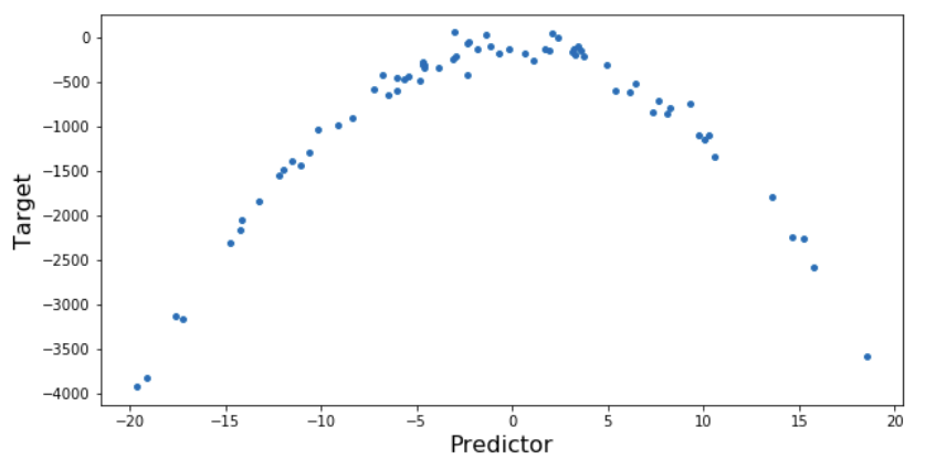
I’m going to take a slightly different approach here. We will implement both the polynomial regression as well as linear regression algorithms on a simple dataset where we have a curvilinear relationship between the target and predictor. Finally, we will compare the results to understand the difference between the two.

First, import the required libraries and plot the relationship between the target variable and the independent variable:

Python Code:

Let’s start with Linear Regression first:

# Importing Linear Regression
from sklearn.linear_model import LinearRegression

# Training Model
lm=LinearRegression()
lm.fit(x.reshape(-1,1),y.reshape(-1,1))

Let’s see how linear regression performs on this dataset:

y_pred=lm.predict(x.reshape(-1,1))

# plotting predictions
plt.figure(figsize=(10,5))
plt.scatter(x,y,s=15)
plt.plot(x,y_pred,color='r')
plt.xlabel('Predictor',fontsize=16)
plt.ylabel('Target',fontsize=16)
plt.show()

print('RMSE for Linear Regression=>',np.sqrt(mean_squared_error(y,y_pred)))

Here, you can see that the linear regression model is not able to fit the data properly and the RMSE (Root Mean Squared Error) is also very high.

Now, let’s try polynomial regression.

The implementation of polynomial regression is a two-step process. First, we transform our data into a polynomial using the PolynomialFeatures function from sklearn and then use linear regression to fit the parameters:

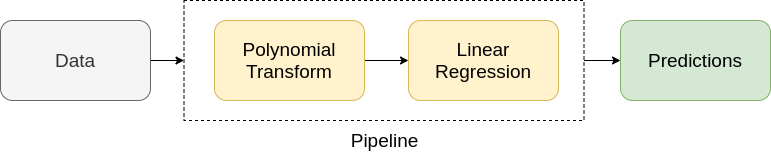
We can automate this process using pipelines. Pipelines can be created using Pipeline from sklearn.

Let’s create a pipeline for performing polynomial regression:

# importing libraries for polynomial transform
from sklearn.preprocessing import PolynomialFeatures
# for creating pipeline
from sklearn.pipeline import Pipeline
# creating pipeline and fitting it on data
Input=[('polynomial',PolynomialFeatures(degree=2)),('modal',LinearRegression())]
pipe=Pipeline(Input)
pipe.fit(x.reshape(-1,1),y.reshape(-1,1))

Here, I have taken a 2-degree polynomial. We can choose the degree of polynomial based on the relationship between target and predictor. The 1-degree polynomial is a simple linear regression; therefore, the value of degree must be greater than 1.

With the increasing degree of the polynomial, the complexity of the model also increases. Therefore, the value of n must be chosen precisely. If this value is low, then the model won’t be able to fit the data properly and if high, the model will overfit the data easily.

Read more about underfitting and overfitting in machine learning here.

Let’s take a look at our model’s performance:

poly_pred=pipe.predict(x.reshape(-1,1))
#sorting predicted values with respect to predictor
sorted_zip = sorted(zip(x,poly_pred))
x_poly, poly_pred = zip(*sorted_zip)
#plotting predictions
plt.figure(figsize=(10,6))
plt.scatter(x,y,s=15)
plt.plot(x,y_pred,color='r',label='Linear Regression')
plt.plot(x_poly,poly_pred,color='g',label='Polynomial Regression')
plt.xlabel('Predictor',fontsize=16)
plt.ylabel('Target',fontsize=16)
plt.legend()
plt.show()

print('RMSE for Polynomial Regression=>',np.sqrt(mean_squared_error(y,poly_pred)))

We can clearly observe that Polynomial Regression is better at fitting the data than linear regression. Also, due to better-fitting, the RMSE of Polynomial Regression is way lower than that of Linear Regression.

But what if we have more than one predictor?

For 2 predictors, the equation of the polynomial regression becomes:

where,

Y is the target,

x1, x2 are the predictors,

𝜃0 is the bias,

and, 𝜃1, 𝜃2, 𝜃3, 𝜃4, and 𝜃5 are the weights in the regression equation

For n predictors, the equation includes all the possible combinations of different order polynomials. This is known as Multi-dimensional Polynomial Regression.

But, there is a major issue with multi-dimensional Polynomial Regression – multicollinearity. Multicollinearity is the interdependence between the predictors in a multiple dimensional regression problem. This restricts the model from fitting properly on the dataset.

End Notes

This was a quick introduction to polynomial regression. I haven’t seen a lot of folks talking about this but it can be a helpful algorithm to have at your disposal in machine learning.

I hope you enjoyed this article. If you found this article informative, then please share it with your friends and comment below with your queries and feedback. I also have listed some great courses related to data science below:

Abhishek Sharma 20 Jun 2022

He is a data science aficionado, who loves diving into data and generating insights from it. He is always ready for making machines to learn through code and writing technical blogs. His areas of interest include Machine Learning and Natural Language Processing still open for something new and exciting.

Beginner Machine Learning Python Regression Structured Data