The Ultimate NumPy Tutorial for Data Science Beginners
Highlights
- NumPy is a core Python library every data science professional should be well acquainted with
- This comprehensive NumPy tutorial covers NumPy from scratch, from basic mathematical operations to how Numpy works with image data
- Plenty of Numpy concepts and Python code in this article
Introduction
I am a huge fan of the NumPy library in Python. I have relied on it countless times during my data science journey to perform all sorts of tasks, from basic mathematical operations to using it for image classification!
In short – NumPy is one of the most fundamental libraries in Python and perhaps the most useful of them all. NumPy handles large datasets effectively and efficiently. I can see your eyes glinting at the prospect of mastering NumPy already. 🙂 As a data scientist or as an aspiring data science professional, we need to have a solid grasp on NumPy and how it works in Python.

In this article, I am going to start off by describing what the NumPy library is and why you should prefer it over the ubiquitous but cumbersome Python lists. Then, we will cover some of the most basic NumPy operations that will get you hooked on to this awesome library!
If you’re new to Python, don’t worry! You can take the comprehensive (and free) Python course to learn everything you need to get started with data science programming!
Here’s how we’ll learn NumPy:
- What is the NumPy Library in Python?
- Python list vs NumPy arrays – What’s the Difference?
- Creating a NumPy Array
- Basic ndarray
- Array of zeros
- Array of ones
- Random numbers in ndarray
- An array of your choice
- Imatrix in NumPy
- Evenly spaced ndarray
- The Shape and Reshaping of NumPy Array
- Dimensions of NumPy array
- Shape of NumPy array
- Size of NumPy array
- Reshaping a NumPy array
- Flattening a NumPy array
- Transpose of a NumPy array
- Expanding and Squeezing a NumPy Array
- Expanding a NumPy array
- Squeezing a NumPy array
- Indexing and Slicing of NumPy Array
- Slicing 1-D NumPy arrays
- Slicing 2-D NumPy arrays
- Slicing 3-D NumPy arrays
- Negative slicing of NumPy arrays
- Stacking and Concatenating Numpy Arrays
- Stacking ndarrays
- Concatenating ndarrays
- Broadcasting in Numpy Arrays – A class apart!
- NumPy Ufuncs – The secret of its success!
- Maths with NumPy Arrays
- Mean, Median and Standard deviation
- Min-Max values and their indexes
- Sorting in NumPy Arrays
- NumPy Arrays and Images
What is the NumPy library in Python?
NumPy stands for Numerical Python and is one of the most useful scientific libraries in Python programming. It provides support for large multidimensional array objects and various tools to work with them. Various other libraries like Pandas, Matplotlib, and Scikit-learn are built on top of this amazing library.
Arrays are a collection of elements/values, that can have one or more dimensions. An array of one dimension is called a Vector while having two dimensions is called a Matrix.
NumPy arrays are called ndarray or N-dimensional arrays and they store elements of the same type and size. It is known for its high-performance and provides efficient storage and data operations as arrays grow in size.
NumPy comes pre-installed when you download Anaconda. But if you want to install NumPy separately on your machine, just type the below command on your terminal:
pip install numpy
Now you need to import the library:
import numpy as np
np is the de facto abbreviation for NumPy used by the data science community.
Python Lists vs NumPy Arrays – What’s the Difference?
If you’re familiar with Python, you might be wondering why use NumPy arrays when we already have Python lists? After all, these Python lists act as an array that can store elements of various types. This is a perfectly valid question and the answer to this is hidden in the way Python stores an object in memory.
A Python object is actually a pointer to a memory location that stores all the details about the object, like bytes and the value. Although this extra information is what makes Python a dynamically typed language, it also comes at a cost which becomes apparent when storing a large collection of objects, like in an array.
Python lists are essentially an array of pointers, each pointing to a location that contains the information related to the element. This adds a lot of overhead in terms of memory and computation. And most of this information is rendered redundant when all the objects stored in the list are of the same type!
To overcome this problem, we use NumPy arrays that contain only homogeneous elements, i.e. elements having the same data type. This makes it more efficient at storing and manipulating the array. This difference becomes apparent when the array has a large number of elements, say thousands or millions. Also, with NumPy arrays, you can perform element-wise operations, something which is not possible using Python lists!
This is the reason why NumPy arrays are preferred over Python lists when performing mathematical operations on a large amount of data.
Creating a NumPy Array
Basic ndarray
NumPy arrays are very easy to create given the complex problems they solve. To create a very basic ndarray, you use the np.array() method. All you have to pass are the values of the array as a list:
This array contains integer values. You can specify the type of data in the dtype argument:
np.array([1,2,3,4],dtype=np.float32)
Output:
Since NumPy arrays can contain only homogeneous datatypes, values will be upcast if the types do not match:
np.array([1,2.0,3,4])
Output:
Here, NumPy has upcast integer values to float values.
NumPy arrays can be multi-dimensional too.
np.array([[1,2,3,4],[5,6,7,8]])
Here, we created a 2-dimensional array of values.
Note: A matrix is just a rectangular array of numbers with shape N x M where N is the number of rows and M is the number of columns in the matrix. The one you just saw above is a 2 x 4 matrix.
Array of zeros
NumPy lets you create an array of all zeros using the np.zeros() method. All you have to do is pass the shape of the desired array:
np.zeros(5)
The one above is a 1-D array while the one below is a 2-D array:
np.zeros((2,3))
np.ones(5,dtype=np.int32)
Random numbers in ndarrays
Another very commonly used method to create ndarrays is np.random.rand() method. It creates an array of a given shape with random values from [0,1):
# random
np.random.rand(2,3)
array([[0.95580785, 0.98378873, 0.65133872],
       [0.38330437, 0.16033608, 0.13826526]])
An array of your choice
Or, in fact, you can create an array filled with any given value using the np.full() method. Just pass in the shape of the desired array and the value you want:
np.full((2,2),7)
Imatrix in NumPy
Another great method is np.eye() that returns an array with 1s along its diagonal and 0s everywhere else.
An Identity matrix is a square matrix that has 1s along its main diagonal and 0s everywhere else. Below is an Identity matrix of shape 3 x 3.
Note: A square matrix has an N x N shape. This means it has the same number of rows and columns.
# identity matrix
np.eye(3)
However, NumPy gives you the flexibility to change the diagonal along which the values have to be 1s. You can either move it above the main diagonal:
# not an identity matrix
np.eye(3,k=1)
Or move it below the main diagonal:
np.eye(3,k=-2)
Note: A matrix is called the Identity matrix only when the 1s are along the main diagonal and not any other diagonal!
Evenly spaced ndarray
You can quickly get an evenly spaced array of numbers using the np.arange() method:
np.arange(5)
The start, end and step size of the interval of values can be explicitly defined by passing in three numbers as arguments for these values respectively. A point to be noted here is that the interval is defined as [start,end) where the last number will not be included in the array:
np.arange(2,10,2)
Alternate elements were printed because the step-size was defined as 2. Notice that 10 was not printed as it was the last element.

Another similar function is np.linspace(), but instead of step size, it takes in the number of samples that need to be retrieved from the interval. A point to note here is that the last number is included in the values returned unlike in the case of np.arange().
np.linspace(0,1,5)
Great! Now you know how to create arrays using NumPy. But its also important to know the shape of the array.
The Shape and Reshaping of NumPy Arrays
Once you have created your ndarray, the next thing you would want to do is check the number of axes, shape, and the size of the ndarray.
Dimensions of NumPy arrays
You can easily determine the number of dimensions or axes of a NumPy array using the ndims attribute:
# number of axis
a = np.array([[5,10,15],[20,25,20]])
print('Array :','\n',a)
print('Dimensions :','\n',a.ndim)
This array has two dimensions: 2 rows and 3 columns.
Shape of NumPy array
The shape is an attribute of the NumPy array that shows how many rows of elements are there along each dimension. You can further index the shape so returned by the ndarray to get value along each dimension:
a = np.array([[1,2,3],[4,5,6]])
print('Array :','\n',a)
print('Shape :','\n',a.shape)
print('Rows = ',a.shape[0])
print('Columns = ',a.shape[1])
Size of NumPy array
You can determine how many values there are in the array using the size attribute. It just multiplies the number of rows by the number of columns in the ndarray:
# size of array
a = np.array([[5,10,15],[20,25,20]])
print('Size of array :',a.size)
print('Manual determination of size of array :',a.shape[0]*a.shape[1])

Reshaping a NumPy array
Reshaping a ndarray can be done using the np.reshape() method. It changes the shape of the ndarray without changing the data within the ndarray:
# reshape
a = np.array([3,6,9,12])
np.reshape(a,(2,2))
Here, I reshaped the ndarray from a 1-D to a 2-D ndarray.
While reshaping, if you are unsure about the shape of any of the axis, just input -1. NumPy automatically calculates the shape when it sees a -1:
a = np.array([3,6,9,12,18,24])
print('Three rows :','\n',np.reshape(a,(3,-1)))
print('Three columns :','\n',np.reshape(a,(-1,3)))
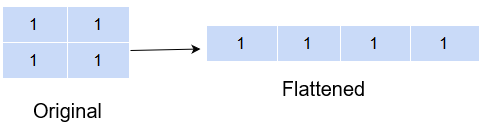
Flattening a NumPy array
Sometimes when you have a multidimensional array and want to collapse it to a single-dimensional array, you can either use the flatten() method or the ravel() method:
a = np.ones((2,2))
b = a.flatten()
c = a.ravel()
print('Original shape :', a.shape)
print('Array :','\n', a)
print('Shape after flatten :',b.shape)
print('Array :','\n', b)
print('Shape after ravel :',c.shape)
print('Array :','\n', c)
Original shape : (2, 2)
Array :
 [[1. 1.]
 [1. 1.]]
Shape after flatten : (4,)
Array :
 [1. 1. 1. 1.]
Shape after ravel : (4,)
Array :
 [1. 1. 1. 1.]
But an important difference between flatten() and ravel() is that the former returns a copy of the original array while the latter returns a reference to the original array. This means any changes made to the array returned from ravel() will also be reflected in the original array while this will not be the case with flatten().
b[0] = 0
print(a)
[[1. 1.]
 [1. 1.]]
The change made was not reflected in the original array.
c[0] = 0
print(a)
[[0. 1.]
 [1. 1.]]
But here, the changed value is also reflected in the original ndarray.
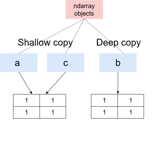
What is happening here is that flatten() creates a Deep copy of the ndarray while ravel() creates a Shallow copy of the ndarray.
Deep copy means that a completely new ndarray is created in memory and the ndarray object returned by flatten() is now pointing to this memory location. Therefore, any changes made here will not be reflected in the original ndarray.
A Shallow copy, on the other hand, returns a reference to the original memory location. Meaning the object returned by ravel() is pointing to the same memory location as the original ndarray object. So, definitely, any changes made to this ndarray will also be reflected in the original ndarray too.
Transpose of a NumPy array
Another very interesting reshaping method of NumPy is the transpose() method. It takes the input array and swaps the rows with the column values, and the column values with the values of the rows:
a = np.array([[1,2,3],
[4,5,6]])
b = np.transpose(a)
print('Original','\n','Shape',a.shape,'\n',a)
print('Expand along columns:','\n','Shape',b.shape,'\n',b)
On transposing a 2 x 3 array, we got a 3 x 2 array. Transpose has a lot of significance in linear algebra.
Expanding and Squeezing a NumPy array
Expanding a NumPy array
You can add a new axis to an array using the expand_dims() method by providing the array and the axis along which to expand:
# expand dimensions
a = np.array([1,2,3])
b = np.expand_dims(a,axis=0)
c = np.expand_dims(a,axis=1)
print('Original:','\n','Shape',a.shape,'\n',a)
print('Expand along columns:','\n','Shape',b.shape,'\n',b)
print('Expand along rows:','\n','Shape',c.shape,'\n',c)
Squeezing a NumPy array
On the other hand, if you instead want to reduce the axis of the array, use the squeeze() method. It removes the axis that has a single entry. This means if you have created a 2 x 2 x 1 matrix, squeeze() will remove the third dimension from the matrix:
# squeeze
a = np.array([[[1,2,3],
[4,5,6]]])
b = np.squeeze(a, axis=0)
print('Original','\n','Shape',a.shape,'\n',a)
print('Squeeze array:','\n','Shape',b.shape,'\n',b)
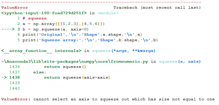
However, if you already had a 2 x 2 matrix, using squeeze() in that case would give you an error:
# squeeze
a = np.array([[1,2,3],
[4,5,6]])
b = np.squeeze(a, axis=0)
print('Original','\n','Shape',a.shape,'\n',a)
print('Squeeze array:','\n','Shape',b.shape,'\n',b)
Indexing and Slicing of NumPy array
So far, we have seen how to create a NumPy array and how to play around with its shape. In this section, we will see how to extract specific values from the array using indexing and slicing.
Slicing 1-D NumPy arrays
Slicing means retrieving elements from one index to another index. All we have to do is to pass the starting and ending point in the index like this: [start: end].
However, you can even take it up a notch by passing the step-size. What is that? Well, suppose you wanted to print every other element from the array, you would define your step-size as 2, meaning get the element 2 places away from the present index.
Incorporating all this into a single index would look something like this: [start:end:step-size].
a = np.array([1,2,3,4,5,6])
print(a[1:5:2])
Notice that the last element did not get considered. This is because slicing includes the start index but excludes the end index.
A way around this is to write the next higher index to the final index value you want to retrieve:
a = np.array([1,2,3,4,5,6])
print(a[1:6:2])
If you don’t specify the start or end index, it is taken as 0 or array size, respectively, as default. And the step-size by default is 1.
a = np.array([1,2,3,4,5,6])
print(a[:6:2])
print(a[1::2])
print(a[1:6:])
Slicing 2-D NumPy arrays
Now, a 2-D array has rows and columns so it can get a little tricky to slice 2-D arrays. But once you understand it, you can slice any dimension array!
Before learning how to slice a 2-D array, let’s have a look at how to retrieve an element from a 2-D array:
a = np.array([[1,2,3],
[4,5,6]])
print(a[0,0])
print(a[1,2])
print(a[1,0])
Here, we provided the row value and column value to identify the element we wanted to extract. While in a 1-D array, we were only providing the column value since there was only 1 row.
So, to slice a 2-D array, you need to mention the slices for both, the row and the column:
a = np.array([[1,2,3],[4,5,6]])
# print first row values
print('First row values :','\n',a[0:1,:])
# with step-size for columns
print('Alternate values from first row:','\n',a[0:1,::2])
#
print('Second column values :','\n',a[:,1::2])
print('Arbitrary values :','\n',a[0:1,1:3])
Slicing 3-D NumPy arrays
So far we haven’t seen a 3-D array. Let’s first visualize how a 3-D array looks like:
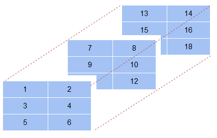
a = np.array([[[1,2],[3,4],[5,6]],# first axis array
[[7,8],[9,10],[11,12]],# second axis array
[[13,14],[15,16],[17,18]]])# third axis array
# 3-D array
print(a)
In addition to the rows and columns, as in a 2-D array, a 3-D array also has a depth axis where it stacks one 2-D array behind the other. So, when you are slicing a 3-D array, you also need to mention which 2-D array you are slicing. This usually comes as the first value in the index:
# value
print('First array, first row, first column value :','\n',a[0,0,0])
print('First array last column :','\n',a[0,:,1])
print('First two rows for second and third arrays :','\n',a[1:,0:2,0:2])
If in case you wanted the values as a single dimension array, you can always use the flatten() method to do the job!
print('Printing as a single array :','\n',a[1:,0:2,0:2].flatten())
Negative slicing of NumPy arrays
An interesting way to slice your array is to use negative slicing. Negative slicing prints elements from the end rather than the beginning. Have a look below:
a = np.array([[1,2,3,4,5],
[6,7,8,9,10]])
print(a[:,-1])
Here, the last values for each row were printed. If, however, we wanted to extract from the end, we would have to explicitly provide a negative step-size otherwise the result would be an empty list.
print(a[:,-1:-3:-1])
Having said that, the basic logic of slicing remains the same, i.e. the end index is never included in the output.
An interesting use of negative slicing is to reverse the original array.
a = np.array([[1,2,3,4,5],
[6,7,8,9,10]])
print('Original array :','\n',a)
print('Reversed array :','\n',a[::-1,::-1])
You can also use the flip() method to reverse an ndarray.
a = np.array([[1,2,3,4,5],
[6,7,8,9,10]])
print('Original array :','\n',a)
print('Reversed array vertically :','\n',np.flip(a,axis=1))
print('Reversed array horizontally :','\n',np.flip(a,axis=0))
Stacking and Concatenating NumPy arrays
Stacking ndarrays
You can create a new array by combining existing arrays. This you can do in two ways:
- Either combine the arrays vertically (i.e. along the rows) using the vstack() method, thereby increasing the number of rows in the resulting array
- Or combine the arrays in a horizontal fashion (i.e. along the columns) using the hstack(), thereby increasing the number of columns in the resultant array
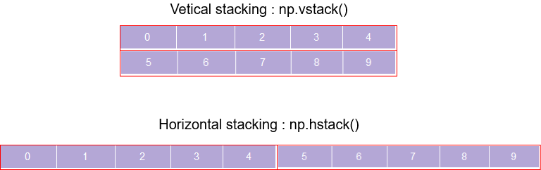
a = np.arange(0,5)
b = np.arange(5,10)
print('Array 1 :','\n',a)
print('Array 2 :','\n',b)
print('Vertical stacking :','\n',np.vstack((a,b)))
print('Horizontal stacking :','\n',np.hstack((a,b)))
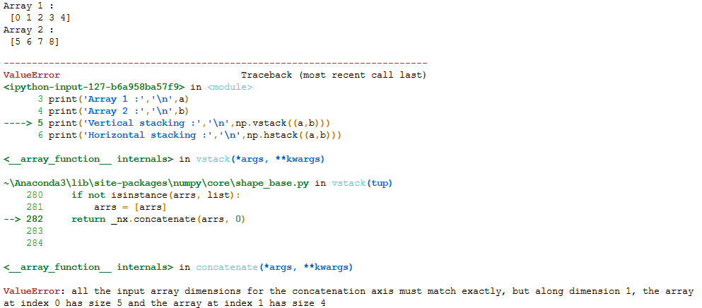
A point to note here is that the axis along which you are combining the array should have the same size otherwise you are bound to get an error!
a = np.arange(0,5)
b = np.arange(5,9)
print('Array 1 :','\n',a)
print('Array 2 :','\n',b)
print('Vertical stacking :','\n',np.vstack((a,b)))
print('Horizontal stacking :','\n',np.hstack((a,b)))
Another interesting way to combine arrays is using the dstack() method. It combines array elements index by index and stacks them along the depth axis:
a = [[1,2],[3,4]]
b = [[5,6],[7,8]]
c = np.dstack((a,b))
print('Array 1 :','\n',a)
print('Array 2 :','\n',b)
print('Dstack :','\n',c)
print(c.shape)

Concatenating ndarrays
While stacking arrays is one way of combining old arrays to get a new one, you could also use the concatenate() method where the passed arrays are joined along an existing axis:
a = np.arange(0,5).reshape(1,5)
b = np.arange(5,10).reshape(1,5)
print('Array 1 :','\n',a)
print('Array 2 :','\n',b)
print('Concatenate along rows :','\n',np.concatenate((a,b),axis=0))
print('Concatenate along columns :','\n',np.concatenate((a,b),axis=1))
The drawback of this method is that the original array must have the axis along which you want to combine. Otherwise, get ready to be greeted by an error.
Another very useful function is the append method that adds new elements to the end of a ndarray. This is obviously useful when you already have an existing ndarray but want to add new values to it.
# append values to ndarray
a = np.array([[1,2],
             [3,4]])
np.append(a,[[5,6]], axis=0)
Broadcasting in NumPy arrays – A class apart!
Broadcasting is one of the best features of ndarrays. It lets you perform arithmetics operations between ndarrays of different sizes or between an ndarray and a simple number!
Broadcasting essentially stretches the smaller ndarray so that it matches the shape of the larger ndarray:
a = np.arange(10,20,2)
b = np.array([[2],[2]])
print('Adding two different size arrays :','\n',a+b)
print('Multiplying an ndarray and a number :',a*2)
Adding two different size arrays :
 [[12 14 16 18 20]
 [12 14 16 18 20]]
Multiplying an ndarray and a number : [20 24 28 32 36]
Its working can be thought of like stretching or making copies of the scalar, the number, [2, 2, 2] to match the shape of the ndarray and then perform the operation element-wise. But no such copies are being made. It is just a way of thinking about how broadcasting is working.
This is very useful because it is more efficient to multiply an array with a scalar value rather than another array! It is important to note that two ndarrays can broadcast together only when they are compatible.
Ndarrays are compatible when:
- Both have the same dimensions
- Either of the ndarrays has a dimension of 1. The one having a dimension of 1 is broadcast to meet the size requirements of the larger ndarray
In case the arrays are not compatible, you will get a ValueError.
a = np.ones((3,3))
b = np.array([2])
a+b
Here, the second ndarray was stretched, hypothetically, to a 3 x 3 shape, and then the result was calculated.
NumPy Ufuncs – The secret of its success!
Python is a dynamically typed language. This means the data type of a variable does not need to be known at the time of the assignment. Python will automatically determine it at run-time. While this means a cleaner and easier code to write, it also makes Python sluggish.
This problem manifests itself when Python has to do many operations repeatedly, like the addition of two arrays. This is so because each time an operation needs to be performed, Python has to check the data type of the element. This problem is overcome by NumPy using the ufuncs function.
The way NumPy makes this work faster is by using vectorization. Vectorization performs the same operation on ndarray in an element-by-element fashion in a compiled code. So the data types of the elements do not need to be determined every time, thereby performing faster operations.
ufuncs are Universal functions in NumPy that are simply mathematical functions. They perform fast element-wise functions. They are called automatically when you are performing simple arithmetic operations on NumPy arrays because they act as wrappers for NumPy ufuncs.
For example, when adding two NumPy arrays using ‘+’, the NumPy ufunc add() is automatically called behind the scene and quietly does its magic:
a = [1,2,3,4,5]
b = [6,7,8,9,10]
%timeit a+b
![]()
a = np.arange(1,6)
b = np.arange(6,11)
%timeit a+b
![]()
You can see how the same addition of two arrays has been done in significantly less time with the help of NumPy ufuncs!
Maths with NumPy arrays
Here are some of the most important and useful operations that you will need to perform on your NumPy array.
Basic arithmetic operations on NumPy arrays
The basic arithmetic operations can easily be performed on NumPy arrays. The important thing to remember is that these simple arithmetics operation symbols just act as wrappers for NumPy ufuncs.
print('Subtract :',a-5)
print('Multiply :',a*5)
print('Divide :',a/5)
print('Power :',a**2)
print('Remainder :',a%5)
Subtract : [-4 -3 -2 -1 0]
Multiply : [ 5 10 15 20 25]
Divide : [0.2 0.4 0.6 0.8 1. ]
Power : [ 1 4 9 16 25]
Remainder : [1 2 3 4 0]
Mean, Median and Standard deviation
To find the mean and standard deviation of a NumPy array, use the mean(), std() and median() methods:
a = np.arange(5,15,2)
print('Mean :',np.mean(a))
print('Standard deviation :',np.std(a))
print('Median :',np.median(a))
Min-Max values and their indexes
Min and Max values in an ndarray can be easily found using the min() and max() methods:
a = np.array([[1,6],
[4,3]])
# minimum along a column
print('Min :',np.min(a,axis=0))
# maximum along a row
print('Max :',np.max(a,axis=1))
You can also easily determine the index of the minimum or maximum value in the ndarray along a particular axis using the argmin() and argmax() methods:
a = np.array([[1,6,5],
[4,3,7]])
# minimum along a column
print('Min :',np.argmin(a,axis=0))
# maximum along a row
print('Max :',np.argmax(a,axis=1))
Let me break down the output for you. The minimum value for the first column is the first element along the column. For the second column, it is the second element. And for the third column, it is the first element.
You can similarly determine what the output for maximum values indicates.
Sorting in NumPy arrays
For any programmer, the time complexity of any algorithm is of prime essence. Sorting is an important and very basic operation that you might well use on a daily basis as a data scientist. So, it is important to use a good sorting algorithm with minimum time complexity.
The NumPy library is a legend when it comes to sorting elements of an array. It has a range of sorting functions that you can use to sort your array elements. It has implemented quicksort, heapsort, mergesort, and timesort for you under the hood when you use the sort() method:
a = np.array([1,4,2,5,3,6,8,7,9])
np.sort(a, kind='quicksort')
You can even sort the array along any axis you desire:
a = np.array([[5,6,7,4],
              [9,2,3,7]])# sort along the column
print('Sort along column :','\n',np.sort(a, kind='mergresort',axis=1))
# sort along the row
print('Sort along row :','\n',np.sort(a, kind='mergresort',axis=0))
NumPy arrays and Images
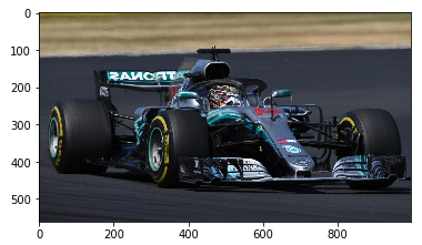
NumPy arrays find wide use in storing and manipulating image data. But what is image data really?
Images are made up of pixels that are stored in the form of an array. Each pixel has a value ranging between 0 to 255 – 0 indicating a black pixel and 255 indicating a white pixel. A colored image consists of three 2-D arrays, one for each of the color channels: Red, Green, and Blue, placed back-to-back thus making a 3-D array. Each value in the array constitutes a pixel value. So, the size of the array depends on the number of pixels along each dimension.
Have a look at the image below:

Python can read the image as an array using the scipy.misc.imread() method in the SciPy library. And when we output it, it is simply a 3-D array containing the pixel values:
import numpy as np
import matplotlib.pyplot as plt
from scipy import misc

# read image
im = misc.imread('./original.jpg')
# image
im
array([[[115, 106,  67],
        [113, 104,  65],
        [112, 103,  64],
        ...,
        [160, 138,  37],
        [160, 138,  37],
        [160, 138,  37]],

       [[117, 108,  69],
        [115, 106,  67],
        [114, 105,  66],
        ...,
        [157, 135,  36],
        [157, 135,  34],
        [158, 136,  37]],

       [[120, 110,  74],
        [118, 108,  72],
        [117, 107,  71],
        ...,
We can check the shape and type of this NumPy array:
print(im.shape)
print(type(type))
(561, 997, 3)
numpy.ndarray
Now, since an image is just an array, we can easily manipulate it using an array function that we have looked at in the article. Like, we could flip the image horizontally using the np.flip() method:
# flip
plt.imshow(np.flip(im, axis=1))
Or you could normalize or change the range of values of the pixels. This is sometimes useful for faster computations.
im/255
array([[[0.45098039, 0.41568627, 0.2627451 ],
        [0.44313725, 0.40784314, 0.25490196],
        [0.43921569, 0.40392157, 0.25098039],
        ...,
        [0.62745098, 0.54117647, 0.14509804],
        [0.62745098, 0.54117647, 0.14509804],
        [0.62745098, 0.54117647, 0.14509804]],

       [[0.45882353, 0.42352941, 0.27058824],
        [0.45098039, 0.41568627, 0.2627451 ],
        [0.44705882, 0.41176471, 0.25882353],
        ...,
        [0.61568627, 0.52941176, 0.14117647],
        [0.61568627, 0.52941176, 0.13333333],
        [0.61960784, 0.53333333, 0.14509804]],

       [[0.47058824, 0.43137255, 0.29019608],
        [0.4627451 , 0.42352941, 0.28235294],
        [0.45882353, 0.41960784, 0.27843137],
        ...,
        [0.6       , 0.52156863, 0.14117647],
        [0.6       , 0.52156863, 0.13333333],
        [0.6       , 0.52156863, 0.14117647]],

       ...,
Remember this is using the same concept of ufuncs and broadcasting that we saw in the article!
There are a lot more things that you could do to manipulate your images that would be useful when you are classifying images using Neural Networks. If you are interested in building your own image classifier, you could head here for an amazing tutorial on the topic!
End Notes
Phew – take a deep breath. We’ve covered a LOT of ground in this article. You are well acquainted with the use of NumPy arrays and are all guns blazing to incorporate it into your daily analysis tasks.
To get to know more about any NumPy function, check out their official documentation where you will find a detailed description of each and every function.
Going forward, I recommend you to explore the following courses on Data Science to help in your journey to becoming an awesome Data Scientist!


First of all, I would like to thank you for putting together a helpful list of all that Numpy can do when it comes to data science. I do have a point to make about the timing section of the article. You show examples using Python's list and Numpy's ufunc add. For the list example you get a mean time of 283 ns For the Numpy example you get a mean time of 1.29 us, or 1,290 ns. This example shows the exact opposite point that is being made, that Numpy ufuncs made things significantly faster. I used the exact same code on my own machine as a double check, and the Numpy example was still slower ( 71 ns for list compared to 431 for Numpy)
It is a nice article, written in a well explained way. I learned a lot from this link. WIth thanks and regards, Kishor Kumar Kumawat
Very informative and helpful 🙂