Understanding Skewness in Data and Its Impact on Data Analysis (Updated 2023)

Introduction

The concept of skewness is baked into our way of thinking. When we look at a visualization, our minds intuitively discern the pattern in that chart, whether we are data scientists or beginners working on a python dataset.

As you might already know, India has more than 50% of its population below the age of 25 and more than 65% below the age of 35. If you plot the distribution of the age of the population of India, you will find that there is a hump on the left side of the distribution, and the right side is comparatively planar. In other words, we can say that there’s a skew toward the end, right?

So even if you haven’t read up on skewness as a data science or analytics professional, you have interacted with the concept on an informal note. And it’s a pretty easy topic in statistics – and yet a lot of folks skim through it in their haste to learn other seemingly complex data science concepts. To me, that’s a mistake. Skewness is a fundamental descriptive statistics concept that everyone in data science and analytics needs to know. In this tutorial, we’ll discuss the concept of skewness in the easiest way possible, one of the important concepts in statistics for data science. So buckle up because you’ll learn a concept that you’ll value during your entire data science career.

Learning Objectives

• You’ll learn about skewness, its types, and its importance in the field of data science.
• You will learn what the coefficient of skewness is and how to calculate it.
• Lastly, you will learn how we can transform skewed data.

What Is Skewness?

Skewness is the measure of the asymmetry of an ideally symmetric probability distribution and is given by the third standardized moment. If that sounds way too complex, don’t worry! Let me break it down for you.

In simple words, skewness is the measure of how much the probability distribution of a random variable deviates from the normal distribution. Now, you might be thinking – why am I talking about normal distribution here?

Well, the normal distribution is the probability distribution without any skewness. You can look at the image below, which shows symmetrical distribution that’s a normal distribution, and you can see that it is symmetrical on both sides of the dashed line. Apart from this, there are two types of skewness:

• Positive Skewness
• Negative Skewness

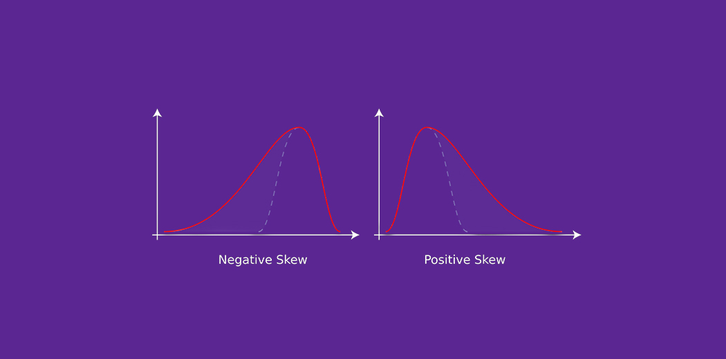
The probability distribution with its tail on the right side is a positively skewed distribution, and the one with its tail on the left side is a negatively skewed distribution. If you’re finding the above figures confusing, that’s alright. We’ll understand this in more detail later.

Skewness is demonstrated on a bell curve when data points are not distributed symmetrically to the left and right sides of the median on a bell curve. If the bell curve is shifted to the left or the right, it is said to be skewed. Before that, let’s understand why this is such an important concept for you as a data science professional.

Why Is Skewness Important?

Now, we know that skewness is the measure of the lack of symmetry, and its types are distinguished by the side on which the tail of probability distribution lies. But why is knowing the skewness of the data important?

First, linear models work on the assumption that the distribution of the independent variable and the target variable are similar. Therefore, knowing about the skewness of data helps us create better linear models.

Secondly, let’s take a look at the below distribution. It is the distribution of horsepower of cars:

You can clearly see that the above distribution is positively skewed. Now, let’s say you want to use this as a feature for the model that will predict the mpg (miles per gallon) of a car.

Since our data is positively skewed here, it means that it has a higher number of data points having low values, i.e., cars with less horsepower. So when we train our model on this data, it will perform better at predicting the mpg of cars with lower horsepower as compared to those with higher horsepower.

Also, skewness tells us about the direction of outliers. You can see that our distribution is positively skewed, and most of the outliers are present on the right side of the distribution.

Note: The skewness does not tell us about the number of outliers. It only tells us the direction.

Now we know why skewness is important, before understanding distributions, let us quickly understand what the central limit theorem is.

Central Limit Theorem

The central limit theorem says that the sampling distribution of the mean will always be normally distributed as long as extreme values or the sample size is large enough. Regardless of whether the population has a normal, Poisson, binomial, or any other distribution, the sampling distribution of the mean will be normal.

Hypothesis Testing uses the Central Limit Theorem. Using the Central Limit Theorem, we can extend the approach employed in Single Sample Hypothesis Testing for normally distributed populations to those that are not normally distributed.

What Is Symmetric/Normal Distribution?

Source: Wikipedia

Yes, we’re back again with the normal distribution. It is used as a reference for determining the skewness of a distribution. As I mentioned earlier, the ideal normal distribution is the probability distribution with almost no skewness. It is nearly perfectly symmetrical. Due to this, the value of skewness for a normal distribution is zero or zero skewness.

But why is it nearly perfectly symmetrical and not absolutely symmetrical?

That’s because, in reality, no real word data has a perfectly normal distribution. Therefore, even the value of skewness is not exactly zero; it is nearly zero. Although the value of zero is used as a reference for determining the skewness of a distribution.

You can see in the above image that the same line represents the mean, median, and mode. It is because the mean, median, and mode of a perfectly normal distribution are equal.

So far, we’ve understood the skewness of normal distribution using a probability or frequency distribution. Now, let’s understand it in terms of a boxplot because that’s the most common way of looking at a distribution in the data science space.

The above image is a boxplot of symmetric distribution. You’ll notice here that the distance between Q1 and Q2 and Q2 and Q3 is equal, i.e.:

But that’s not enough to conclude if a distribution is skewed or not. We also take a look at the length of the whisker; if they are equal, then we can say that the distribution is symmetric, i.e., it is not skewed.

It’s now time to learn about the two types of skewness which we discussed earlier. Let’s start with positive skewness.

Understanding Positively Skewed Distribution | Positive Skewness

Source: Wikipedia

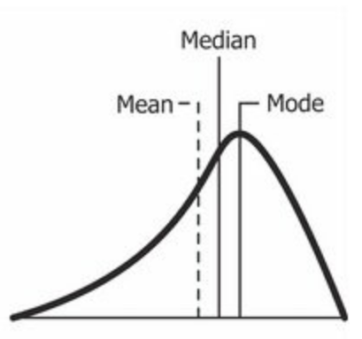
A positive skewness is the right-skewed distribution with the long tail on its right side. The value of skewness for a positively skewed distribution is greater than zero. As you might have already understood by looking at the figure, the value of the mean is the greatest one, followed by the median and then by mode.

So why is this happening?

Well, the answer to that is that the skewness of the data distribution is on the right; it causes the mean to be greater than the median and eventually move to the right. Also, the mode occurs at the highest frequency of the distribution, which is on the left side of the median. Therefore, the measure of central tendencies is mode < median < mean.

In the above boxplot, you can see that Q2 is present nearer to Q1. This represents a positively skewed distribution. In terms of quartiles, it can be given by:

In this case, it was very easy to tell if the data was skewed or not. But what if we have something like this:

Here, Q2-Q1 and Q3-Q2 are equal, and yet the distribution is positively skewed. The keen-eyed among you will have noticed the length of the right whisker is greater than the left whisker. From this, we can conclude that the data is positively skewed.

So, the first step is always to check the equality of Q2-Q1 and Q3-Q2. If that is found equal, then we look for the length of the whiskers.

Note: A high level of skewness or highly skewed data can generate misleading results from statistical tests. Extreme positive skewness is not desirable for a distribution.

Understanding Negatively Skewed Distribution | Negative Skewness

Source: Wikipedia

As you might have already guessed, a negatively skewed distribution is the left-skewed distribution with the long tail on its left side. The value of skewness for a negatively skewed distribution is less than zero. You can also see in the above figure that the measure of central tendencies is mean < median < mode.

In the boxplot, the relationship between quartiles for a negative skewness is given by:

Similar to what we did earlier, if Q3-Q2 and Q2-Q1 are equal, then we look for the length of whiskers. And if the length of the left whisker is greater than that of the right whisker, then we can say that the data is negatively skewed.

Coefficient of Skewness

Pearson developed two methods to find skewness in a sample.

1. Pearson’s Coefficient of Skewness using mode.
   SK1= Mean- mode/ sd
   where sd is the standard deviation for the sample.
2. Pearson’s Coefficient of Skewness using the median.
   SK2=3(mean-median)/sd
   where sd is the standard deviation for the sample. It is generally used when the mode is unknown.

Note: There isn’t an Excel function to find Pearson’s coefficient of skewness. In the descriptive statistics area of the data analysis tool, skewness is calculated by using the third power of deviations around the mean. This is different from Pearson’s coefficient of skewness, which uses either the mode or the mean.

How Do We Transform Skewed Data?

Since you know how much the skewed data can affect our machine learning model’s predicting capabilities, it is better to transform the skewed data into normally distributed data. Here are some of the ways you can transform your skewed data:

• Power Transformation
• Log Transformation
• Exponential Transformation

Note: The selection of transformation depends on the statistical characteristics of the data.

Conclusion

Skewness is a measure of lack of symmetry. It is a shape parameter that characterizes the degree of asymmetry of a distribution. A distribution is said to be positively skewed with a degree of skewness greater than 0 when the tail of a distribution is toward the high values indicating an excess of low values. Conversely, it is negatively skewed with a degree of skewness less than 0 (Sk<0)when the tail of the distribution is toward the low values indicating an excess of high values.

Key Takeaways

• Skewness is a measure of the lack of symmetry in a distribution. A distribution is asymmetrical when its left and right sides are not mirror images.
• In this article, we covered the concept of skewness and learned the difference between positively skewed and negatively skewed distribution.
• We can transform skewed data using Power, Log, and Exponential Transformations.

Frequently Asked Questions