A Detailed Study of Self Supervised Contrastive Loss and Supervised Contrastive Loss
Introduction
Supervised Contrastive Learning paper claims a big deal about supervised learning and cross-entropy loss vs supervised contrastive loss for better image representation and classification tasks. Let’s go in-depth in this paper what is about.
Claim actually close to 1% improvement on image net data set¹.
Self-Supervised Contrastive Learning (SSCL)
Self-Supervised Contrastive Learning (SSCL) utilizes noise contrastive estimation, cosine similarity, and training data to distinguish between similar and dissimilar pairs. By optimizing distance measures, SSCL extracts meaningful representations without explicit labels, making it invaluable for Self supervised learning in diverse domains like computer vision and natural language processing.

Supervised Contratisive Diagram
Architecture wise, its a very simple network resnet 50 having a 128-dimensional head. If you want you can add a few more layers as well.

Codeself.encoder = resnet50()self.head = nn.Linear(2048, 128)def forward(self, x): feat = self.encoder(x) #normalizing the 128 vector is required feat = F.normalize(self.head(feat), dim=1) return feat
As shown in the figure training is done in two-stage.
- Train using contrastive loss (two variations)
- freeze the learned representations and then learn a classifier on a linear layer using a softmax loss. (From the paper)
The above is pretty self explanatory.
Loss, the main flavor of this paper is understanding the self-supervised contrastive loss and supervised contrastive loss.
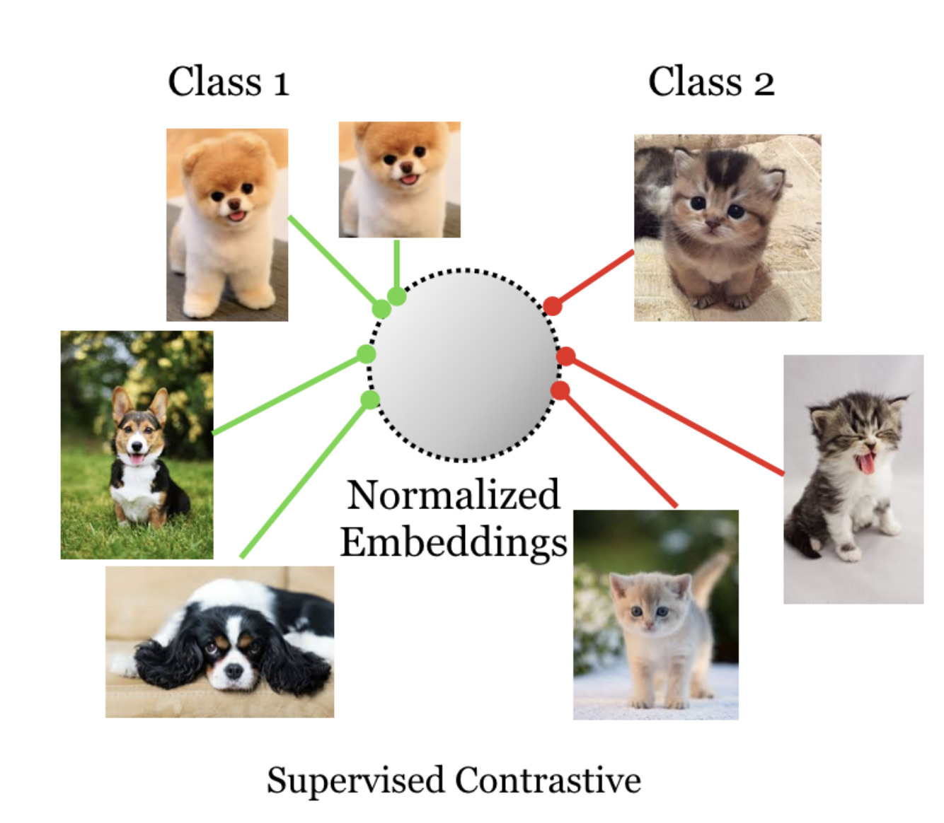
As you can see from the above diagram¹ in SCL (supervised contrastive Loss), a cat is contrasted with any noncat. which means all cats belong to the same label and work as a positive pair and anything noncat is negative. This is very similar to triplet Data and how triplet loss² works.
In case you confused every cat images will be augmented also every-time so even from a single cat image we will have lots of cats.
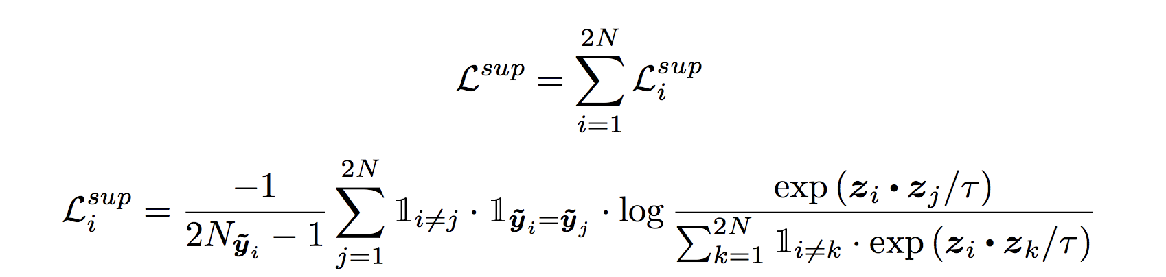
Loss Function For Supervised Contrastive Loss
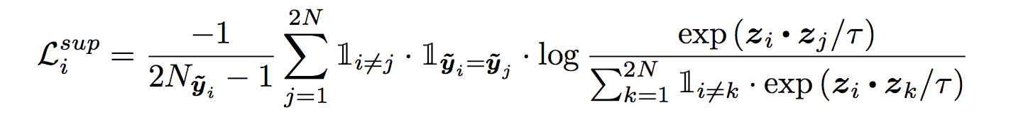
Loss Function for supervised contrastive loss, although it looks monster it’s actually quite simple.
We will see some code later but first very simple explanation. every z is 128 dimensional vector which are normalised.
which means ||z|| =1 Just to reiterate fact from Linear Algebra if u and v two vectors are normalised implies u.v = cos(angel between u and v) which means if two normalised vector are same the dot product between them = 1 # try the below code to convince your selfimport numpy as np v = np.random.randn(128) v = v/np.linalg.norm(v) print(np.dot(v,v)) print(np.linalg.norm(v))
The loss function is with the assumption that every image has one augmentation, N images in a batch create a batch size = 2*N
Read the section of the paper “Generalisation to an arbitrary number of positives”¹
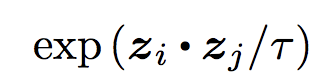
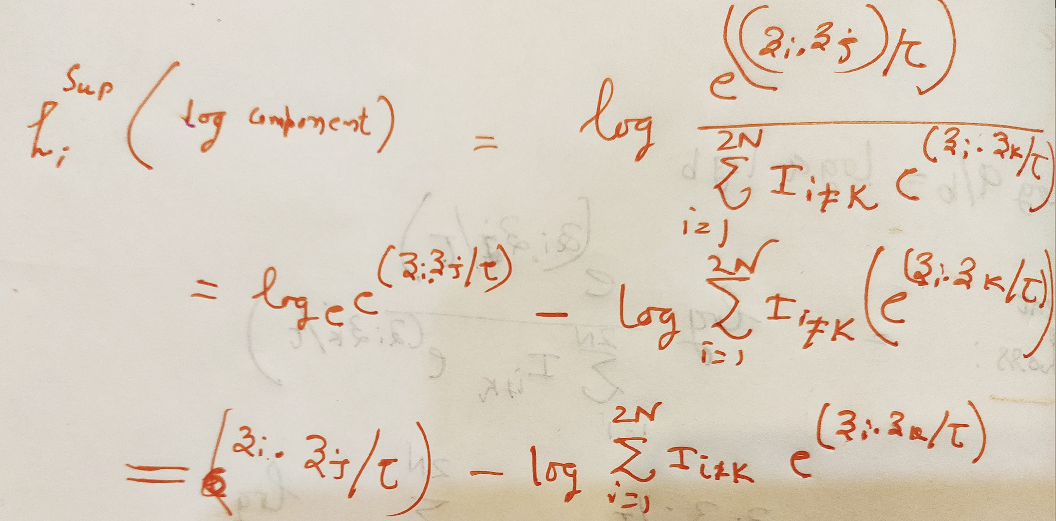
Numerator exp(zi.zj)/tau is a representation of all cats in a batch. Take dot product of zi which is the 128 dim vector of ith image representation with all the j^th 128 dim vectors such that their label is the same and i!=j.
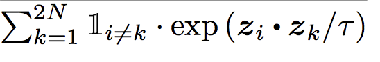
The denominator is ith cat image is dotted with everything else as long it’s not the same cat image. Take the dot of zi and zk such that i!=k means it’s dotted with every image except itself.
Finally, we take the log probability and sum it overall cat images in the batch except itself and divide by 2*N-1
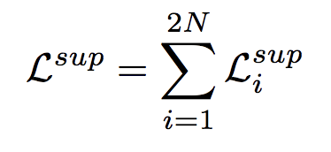
Total Loss sum of losses for all images
Code Let’s understand the above using some torch code.
Let’s assume our batch size is 4 and let’s see how to calculate this loss for a single batch.
For a batch size of 4, your input to the network will be 8x3x224x224 where I have taken image width and height 224.
The reason for 8 = 4X2 as we always have one contrast for each image, one needs to write a data loader accordingly.
The Super contrastive resnet will output you a dimension 8×128 lets split those properly for calculating the batch loss.#batch_size bs = 4
Numerator Code lets calculate this part
temperature = 0.07anchor_feature = contrast_feature#Note we not doing exp their is a reason see below anchor_dot_contrast = torch.div( torch.matmul(anchor_feature, contrast_feature.T), temperature)
Anchor Dot Contrast in case you confused, our feature shapes are 8×128, lets take a 3×128 matrix and the transpose of that and dot them, see the below picture if you can visualize.
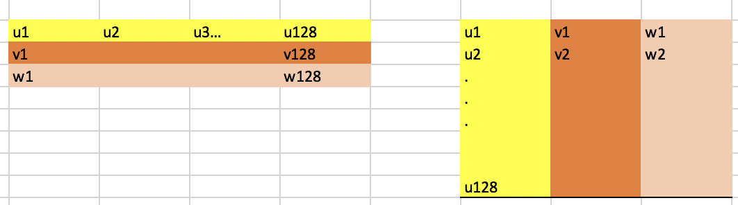
anchor_feature = 3×128 contrast_feature = 128×3 result is 3×3 as below
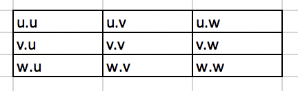
If you notice all diagonal elements are dot with themselves which we don’t want we will get rid of them next.
Linear Algebra fact if u and v are two vectors then u.v is maximum when u = v. So in each row if we take the max of anchor_dot_contrast and negate the same all diagonal will become 0.
Let’s drop the dimension from 128 to 2 to better see this and batch size of 1.#resnet output just mind you i am not normalizing but according to paper you need to use normalize look into torch Functional.#bs 1 and dim 2 means 2*1×2 features = torch.randn(2, 2)temperature = 0.07 contrast_feature = features anchor_feature = contrast_feature anchor_dot_contrast = torch.div( torch.matmul(anchor_feature, contrast_feature.T), temperature) print(‘anchor_dot_contrast=\n{}’.format(anchor_dot_contrast))logits_max, _ = torch.max(anchor_dot_contrast, dim=1, keepdim=True) print(‘logits_max = {}’.format(logits_max)) logits = anchor_dot_contrast – logits_max.detach() print(‘ logits = {}’.format(logits))#output see what happen to diagonalanchor_dot_contrast= tensor([[128.8697, -12.0467], [-12.0467, 50.5816]]) logits_max = tensor([[128.8697], [ 50.5816]]) logits = tensor([[ 0.0000, -140.9164], [ -62.6283, 0.0000]])
Mask. Artificial label creation and creating an appropriate mask for contrastive calculation. This code is a little tricky, so check the output carefully.bs = 4 print(‘batch size’, bs) temperature = 0.07 labels = torch.randint(4, (1,4)) print(‘labels’, labels) mask = torch.eq(labels, labels.T).float() print(‘mask = \n{}’.format(logits_mask))#hard coding it for easier understanding otherwise its features.shape[1] contrast_count = 2 anchor_count = contrast_countmask = mask.repeat(anchor_count, contrast_count)# mask-out self-contrast cases logits_mask = torch.scatter( torch.ones_like(mask), 1, torch.arange(bs * anchor_count).view(-1, 1), 0 ) mask = mask * logits_mask print(‘mask * logits_mask = \n{}’.format(mask))
Let’s understand the output.batch size 4 labels tensor([[3, 0, 2, 3]])#what above means in this perticuler batch of 4 we got 3,0,2,3 labels. Just in case you forgot we are contrasting here only once so we will have 3_c, 0_c, 2_c, 3_c as our contrast in the input batch. #basically batch_size X contrast_count X C x Width X height -> check above if you confusedmask = tensor([[0., 1., 1., 1., 1., 1., 1., 1.], [1., 0., 1., 1., 1., 1., 1., 1.], [1., 1., 0., 1., 1., 1., 1., 1.], [1., 1., 1., 0., 1., 1., 1., 1.], [1., 1., 1., 1., 0., 1., 1., 1.],Easy to understand the Self Supervised Contrastive Loss now which is simpler than this. [1., 1., 1., 1., 1., 0., 1., 1.], [1., 1., 1., 1., 1., 1., 0., 1.], [1., 1., 1., 1., 1., 1., 1., 0.]])#this is really important so we created a mask = mask * logits_mask which tells us for 0 th image representation which are the image it should be contrasted with.# so our labels are labels tensor([[3, 0, 2, 3]]) # I am renaming them for better understanding tensor([[3_1, 0_1, 2_1, 3_2]]) # so at 3_0 will be contrasted with its own augmentation which is at position 5 (index = 4) and position 8 (index = 7) in the first row those are the position marked one else its zero See the image bellow for better understandingmask * logits_mask = tensor([[0., 0., 0., 1., 1., 0., 0., 1.], [0., 0., 0., 0., 0., 1., 0., 0.], [0., 0., 0., 0., 0., 0., 1., 0.], [1., 0., 0., 0., 1., 0., 0., 1.], [1., 0., 0., 1., 0., 0., 0., 1.], [0., 1., 0., 0., 0., 0., 0., 0.], [0., 0., 1., 0., 0., 0., 0., 0.], [1., 0., 0., 1., 1., 0., 0., 0.]])

Anchor dot contrast if you remember from above as below.logits = anchor_dot_contrast — logits_max.detach()
Loss again
Math recap
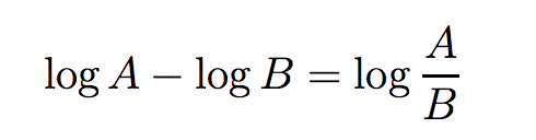
We already have the first part dot product divided by tau as logits.#second part of the above equation equal to torch.log(exp_logits.sum(1, keepdim=True))exp_logits = torch.exp(logits) * logits_mask log_prob = logits – torch.log(exp_logits.sum(1, keepdim=True))# compute mean of log-likelihood over positive mean_log_prob_pos = (mask * log_prob).sum(1) / mask.sum(1)# loss loss = – mean_log_prob_posloss = loss.view(anchor_count, 4).mean() print(’19. loss {}’.format(loss))
I think that’s about the supervised contrastive loss. I think it’s very easy to understand the Self Supervised Contrastive Loss now which is simpler than this.
According to the paper, more contrast_count makes a better model which is self-explanatory. Need to modify the loss function for more than 2 contrast count, hope you can try it with the help of the above explanation.
How does Contrastive Learning work in Vision AI?
Contrastive learning in vision AI involves training a neural network to learn representations of images by maximizing the similarity between similar images and minimizing the similarity between dissimilar ones. Here’s how it typically works:
Positive and Negative Pairs: Each pair of images consists of a positive sample, which depicts similar content (e.g., different views of the same object), and a negative sample, which portrays dissimilar content (e.g., images of different objects). This framework incorporates both positive and negative samples to guide the learning process effectively.
Feature Extraction: Each image undergoes feature extraction through a neural network, often termed as the encoder or backbone network. This process generates a feature vector representing the image, facilitating subsequent comparison and analysis.
Contrastive Learning Objective: The core objective is to enhance the similarity between feature vectors of positive pairs while encouraging dissimilarity among those of negative pairs. This optimization is achieved by employing loss functions tailored for contrastive learning, such as the contrastive loss proposed by Hadsell et al. (2006) or the InfoNCE loss utilized in recent advancements like SimCLR.
Training: During the training phase, the network is supplied with pairs of images alongside their corresponding labels (positive or negative). Through iterative adjustments to its parameters, the network minimizes the contrastive loss, thus acquiring the ability to discern similarities and differences among images.
Evaluation: Once trained, the acquired representations can be leveraged across diverse downstream tasks, including image classification, object detection, and semantic segmentation. These learned representations often exhibit favorable characteristics such as improved generalization and resilience to variations in input data.
In summary, contrastive learning enables the network to derive meaningful image representations autonomously, without the need for explicit supervision. This approach leads to enhanced performance across a broad spectrum of vision-related tasks, underpinning its significance in the realm of computer vision.
Supervised Contrastive Learning
Supervised Contrastive Learning is a machine learning technique that aims to learn representations by contrasting positive pairs (similar instances) against negative pairs (dissimilar instances) in a supervised setting, focusing on “sentence representation learning,” “triplet loss,” “same class,” and “contrastive learning methods.” Unlike unsupervised contrastive learning, where the model learns from raw data without any labeled information, supervised contrastive learning leverages labeled data to guide the learning process.
In supervised contrastive learning, the objective is to maximize the agreement between representations of positive pairs while minimizing the agreement between representations of negative pairs. This is typically achieved by defining a contrastive loss function such as “triplet loss” that encourages similar instances to have representations that are close together in the embedding space, while pushing representations of dissimilar instances farther apart.
Supervised contrastive learning has been shown to be effective in various tasks such as image classification, object detection, and natural language processing, thanks to its utilization of “machine learning technique” and “deep learning.” It often leads to improved performance compared to traditional supervised learning approaches by learning more informative and discriminative representations.
References
- [1] : Supervised Contrastive Learning
- [2] : Florian Schroff, Dmitry Kalenichenko, and James Philbin. Facenet: A unified embedding for face recognition and clustering. In Proceedings of the IEEE conference on computer vision and pattern recognition, pages 815–823, 2015.
- [3] : A Simple Framework for Contrastive Learning of Visual Representations, Ting Chen, Simon Kornblith, Mohammad Norouzi, Geoffrey Hinton
- [4] : https://github.com/google-research/simclr


