Hyperopt: The Alternative Hyperparameter Optimization Technique You Need to Know
Introduction
When working on a machine learning project, you need to follow a series of steps until you reach your goal. One of the pivotal steps in this process is hyperparameter optimization, which is executed after you have selected your model. The model selection process involves evaluating various algorithms to identify the best model that outperforms others based on certain performance metrics.
Once the best model is chosen, the next step is to refine it to achieve its optimal performance. This refinement process, known as hyperparameter optimization, is crucial because even the most promising model can fall short of its potential if its hyperparameters are not tuned correctly. It’s an iterative process that involves systematically searching through multiple combinations of hyperparameter values to find the set that results in the best model performance.

Table of Contents
What is Hyperparameter Optimization?
Before I define hyperparameter optimization you need to understand what is a hyperparameter. In short, hyperparameters are different parameter values that are used to control the learning process and have a significant effect on the performance of machine learning models. Example of hyperparameters in the Random Forest algorithm is the number of estimators (n_estimators), maximum depth(max_depth), and criterion. These parameters are tunable and can directly affect how well the model trains.
Then hyperparameter optimization is a process of finding the right combination of hyperparameter values in order to achieve maximum performance on the data in a reasonable amount of time. It plays a vital role in the prediction accuracy of a machine learning algorithm. Therefore Hyperparameter optimization is considered the trickiest part of building machine learning models.
Most of these machine learning algorithms come with the default hyperparameter values. The default values do not always perform well on different types of Machine Learning projects you have, that is why you need to optimize them in order to get the right combination that will give you the best performance.
A good choice of hyperparameters can really make an algorithm shine.
There are some common strategies for optimizing hyperparameters:
(a) Grid Search
This is a widely used traditional method that performs hyperparameter tuning in order to determine the optimal values for a given model. The Grid search works by trying every possible combination of parameters you want to try in your model, this means it will take a lot of time to perform the entire search which can get very computationally expensive.
NB: You can learn how to implement Grid Search here.
(b) Random Search
This method works differently where random combinations of the values of the hyperparameters are used to find the best solution for the built model. The drawback of Random Search is sometimes misses important points(values) in the search space.
NB: You can learn more about implementing Random Search here.
Alternative Hyperparameter Optimization Techniques
In this series of articles, I will introduce to you different alternative advanced hyperparameter optimization techniques/methods that can help you obtain the best parameters for a given model. We will look at the following techniques.
- Hyperopt
- Scikit Optimize
- Optuna
In this article, I will focus on the implementation of Hyperopt.
If you’re not performing hyperparameter optimization, you need to start now.
What is Hyperopt?
Hyperopt is a powerful Python library for hyperparameter optimization developed by James Bergstra. Hyperopt uses a form of Bayesian optimization for parameter tuning that allows you to get the best parameters for a given model. It can optimize a model with hundreds of parameters on a large scale.
Features of Hyperopt
Hyperopt contains 4 important features you need to know in order to run your first optimization.
(a) Search Space
The hyperopt has different functions to specify ranges for input parameters, these are stochastic search spaces. The most common options for a search space to choose from are:
- hp.choice(label, options) — This can be used for categorical parameters, it returns one of the options, which should be a list or tuple. Example: hp.choice(“criterion”, [“gini”,”entropy”,])
- hp.randint(label, upper) — This can be used for Integer parameters, it returns a random integer in the range (0, upper).Example: hp.randint(“max_features”,50)
- hp.uniform(label, low, high) — It returns a value uniformly between
lowandhighExample: hp.uniform(“max_leaf_nodes”,1,10)
Other options you can use are:
- hp.normal(label, mu, sigma) — This returns a real value that’s normally distributed with mean mu and standard deviation sigma
- hp.qnormal(label, mu, sigma, q) — This returns a value like round(normal(mu, sigma) / q) * q
- hp.lognormal(label, mu, sigma) — This returns a value drawn according to exp(normal(mu, sigma))
- hp.qlognormal(label, mu, sigma, q) — This returns a value like round(exp(normal(mu, sigma)) / q) * q
You can learn more about search space options here.
NB: Every optimizable stochastic expression has a label (e.g., n_estimators) as the first argument. These labels are used to return parameter choices to the caller during the optimization process.
(b) Objective Function
This is a function to minimize that receives hyperparameter values as input from the search space and returns the loss. This means during the optimization process, we train the model with selected hyperparameter values, predict the target feature, and then evaluate the prediction error and give it back to the optimizer. The optimizer will decide which values to check and iterate again. You will learn how to create an objective function in a practical example.
(c) fmin
The fmin function is the optimization function that iterates on different sets of algorithms and their hyperparameters and then minimizes the objective function. the fmin takes 5 inputs which are:-
- The objective function to minimize
- The defined search space
- The search algorithm to use such as Random search, TPE (Tree Parzen Estimators), and Adaptive TPE.
NB:hyperopt.rand.suggestandhyperopt.tpe.suggestprovides logic for a sequential search of the hyperparameter space. - The maximum number of evaluations.
- The trials object (optional).
Example:
fPython Code:
(d) Trial Object
The Trials object is used to keep All hyperparameters, loss, and other information, this means you can access them after running optimization. Also, trials can help you to save important information and later load and then resume the optimization process. (you will learn more in the practical example).
from hyperopt import Trials

trials = Trials()
After understanding the important features of Hyperopt, the way to use Hyperopt is described in the following steps.
- Initialize the space over which to search.
- Define the objective function.
- Select the search algorithm to use.
- Run hyperopt function.
- Analyze the evaluation outputs stored in the trials object.
Hyperopt in Practice
Now that you know the important features of Hyperopt, in this practical example, we will use the Mobile Price Dataset and the task is to create a model that will predict how high the price of the mobile is 0(low cost) or 1(medium cost) or 2(high cost) or 3(very high cost).
Step 1: Install Hyperopt
You can install hyperopt from PyPI.
pip install hyperopt
Then import important packages including Hyperopt.
# import packages
import numpy as np
import pandas as pd
from sklearn.ensemble import RandomForestClassifier
from sklearn import metrics
from sklearn.model_selection import cross_val_score
from sklearn.preprocessing import StandardScaler
from hyperopt import tpe, hp, fmin, STATUS_OK,Trials
from hyperopt.pyll.base import scope

import warnings
warnings.filterwarnings("ignore")
Step 2: Load the Dataset
Let’s load the dataset from the data directory. To get more information about the dataset read here.
# load data
data = pd.read_csv("data/mobile_price_data.csv")
Check the first five rows of the dataset.
#read data

data.head()
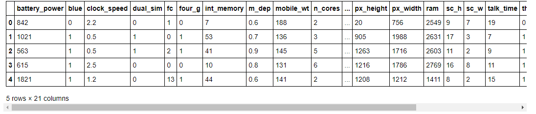
As you can see, in our dataset we have different features with numerical values.
Let’s observe the shape of the dataset.
#show shape

data.shape
(2000, 21)
In this dataset, we have 2000 rows and 21 columns. Now let’s understand the list of features we have in this dataset.
#show list of columns

list(data.columns)
[‘battery_power’, ‘blue’, ‘clock_speed’, ‘dual_sim’, ‘fc’, ‘four_g’, ‘int_memory’, ‘m_dep’, ‘mobile_wt’, ‘n_cores’, ‘pc’, ‘px_height’, ‘px_width’, ‘ram’, ‘sc_h’, ‘sc_w’, ‘talk_time’, ‘three_g’, ‘touch_screen’, ‘wifi’, ‘price_range’]
You can find the meaning of each column name here.
Step 3: Split the Dataset into Target Features and Independent Features
This is a classification problem, we will then split the target feature and independent features from the dataset. Our target feature is price_range.
# split data into features and target

X = data.drop("price_range", axis=1).values
y = data.price_range.values
Step 4: Preprocess the Dataset
Then standardize the independent features by using the StandardScaler method from scikit-learn.
# standardize the feature variables

scaler = StandardScaler()
X_scaled = scaler.fit_transform(X)
Step 5: Define Parameter Space for Optimization
We will use three hyperparameters of the Random Forest algorithm which are n_estimators,max_depth, and criterion.
space = {
    "n_estimators": hp.choice("n_estimators", [100, 200, 300, 400,500,600]),
    "max_depth": hp.quniform("max_depth", 1, 15,1),
    "criterion": hp.choice("criterion", ["gini", "entropy"]),
}
We have set different values in the above-selected hyperparameters. Then we will define the objective function.
Step 6: Define a Function to Minimize (Objective Function)
Our function to minimize is called hyperparamter_tuning and the classification algorithm to optimize its hyperparameter is Random Forest. I use cross-validation to avoid overfitting and then the function will return a loss values and its status.
# define objective function

def hyperparameter_tuning(params):
    clf = RandomForestClassifier(**params,n_jobs=-1)
    acc = cross_val_score(clf, X_scaled, y,scoring="accuracy").mean()
    return {"loss": -acc, "status": STATUS_OK}
NB: Remember that hyperopic minimizes the function, that why I add a negative sign in the acc :
Step 7: Fine Tune the Model
Finally first instantiate the Trial object, fine-tuning the model, and then print the best loss with its hyperparameters values.
# Initialize trials object
trials = Trials()

best = fmin(
    fn=hyperparameter_tuning,
    space = space,
    algo=tpe.suggest,
    max_evals=100,
    trials=trials
)

print("Best: {}".format(best))
100%|█████████████████████████████████████████████████████████| 100/100 [10:30<00:00, 6.30s/trial, best loss: -0.8915] Best: {‘criterion’: 1, ‘max_depth’: 11.0, ‘n_estimators’: 2}.
After performing hyperparameter optimization, the loss is -0.8915 means the model performance has an accuracy of 89.15% by using n_estimators = 300,max_depth = 11, and criterion = “entropy” in the Random Forest classifier.
Step 8: Analyze Results Using Trial Object
The trial object can help us to inspect all of the return values that were calculated during the experiment.
(a) trials.results
This shows a list of dictionaries returned by ‘objective’ during the search.
trials.results
[{‘loss’: -0.8790000000000001, ‘status’: ‘ok’}, {‘loss’: -0.877, ‘status’: ‘ok’}, {‘loss’: -0.768, ‘status’: ‘ok’}, {‘loss’: -0.8205, ‘status’: ‘ok’}, {‘loss’: -0.8720000000000001, ‘status’: ‘ok’}, {‘loss’: -0.883, ‘status’: ‘ok’}, {‘loss’: -0.8554999999999999, ‘status’: ‘ok’}, {‘loss’: -0.8789999999999999, ‘status’: ‘ok’}, {‘loss’: -0.595, ‘status’: ‘ok’},…….]
(b) trials.losses()
This shows a list of losses (float for each ‘ok’ trial).
trials.losses()
[-0.8790000000000001, -0.877, -0.768, -0.8205, -0.8720000000000001, -0.883, -0.8554999999999999, -0.8789999999999999, -0.595, -0.8765000000000001, -0.877, ………]
(c) trials.statuses()
This shows a list of status strings.
trials.statuses()
[‘ok’, ‘ok’, ‘ok’, ‘ok’, ‘ok’, ‘ok’, ‘ok’, ‘ok’, ‘ok’, ‘ok’, ‘ok’, ‘ok’, ‘ok’, ‘ok’, ‘ok’, ‘ok’, ‘ok’, ‘ok’, ‘ok’, ……….]
NB: This trial object can be saved, passed on to the built-in plotting routines, or analyzed with your own custom code.
HyperOpt vs. HyperOpt-Sklearn
While HyperOpt is a powerful and versatile library for hyperparameter optimization, it requires more manual configuration and coding compared to other options. This is where HyperOpt-Sklearn comes in.
HyperOpt-Sklearn is a wrapper built on top of HyperOpt that specifically targets scikit-learn models. It offers several advantages:
- Simplified API: HyperOpt-Sklearn uses a familiar scikit-learn-like API, making it easier to use for those already comfortable with the library.
- Automatic search space definition: It automatically extracts hyperparameters from scikit-learn models, eliminating the need for manual specification.
- Integration with scikit-learn pipelines: It seamlessly integrates with scikit-learn pipelines, allowing you to optimize hyperparameters within your existing workflow.
However, HyperOpt-Sklearn also has limitations:
- Less flexibility: It is less flexible than HyperOpt, as it is specifically designed for scikit-learn models.
- Limited search algorithms: It offers a smaller set of search algorithms compared to HyperOpt.
Choosing between HyperOpt and HyperOpt-Sklearn:
- Use HyperOpt: If you need maximum flexibility and control over your optimization process, or if you are working with non-scikit-learn models, choose HyperOpt.
- Use HyperOpt-Sklearn: If you are using scikit-learn models and prefer a simpler, more user-friendly API, choose HyperOpt-Sklearn.
Conclusion
Congratulations, you have made it to the end of this article! Concluding our exploration of Hyperopt, a beacon in the realm of hyperparameter optimization, we’ve uncovered a compelling alternative to traditional methods. Hyperopt, with its Bayesian optimization prowess, transforms the daunting task of parameter tuning into an efficient quest for excellence.
Our journey through the Mobile Price Dataset demonstrated Hyperopt’s ability to elevate model performance, showcasing its strategic optimization capabilities. The practical example highlighted not only the power of Hyperopt but also its potential to revolutionize model accuracy through optimal parameter selection.
As we wrap up, let’s embrace Hyperopt as our ally in the quest for machine learning mastery, leveraging its innovative approach to unlock the full potential of our models. In the dynamic field of machine learning, Hyperopt stands out as a crucial tool for those aspiring to optimize their models to perfection.
You can download the dataset and notebooks used in this article here:
https://github.com/Davisy/Hyperparameter-Optimization-Techniques
Frequently Asked Questions
A. The “random_state” parameter ensures reproducibility in Hyperopt’s optimization process, allowing for deterministic and repeatable searches by controlling the randomness of the hyperparameter selection.
A. Hyperopt generally operates without explicit gradient information, focusing on black-box optimization. However, when integrated with libraries like Scipy, gradient information can be utilized for more efficient optimization in certain scenarios.
A. Yes, Hyperopt can be integrated with Apache Spark via its API to perform distributed hyperparameter optimization, leveraging Spark’s distributed computing capabilities to speed up the search process.
Hyperopt uses “true” and “false” outcomes to refine its search strategy, focusing on more promising hyperparameter combinations and avoiding areas of the search space that lead to unsuccessful trials.
A. “Args” and “kwargs” allow for the customization of the objective function in Hyperopt, including specifying data splitting strategies through “test_split” to optimize hyperparameters based on model performance across different data splits.
A. Gaussian process models enable Hyperopt to infer the landscape of the objective function, guiding the search toward optimal hyperparameters by estimating the performance of untested combinations without needing direct gradient calculations.


Great blog with good informative content. Keep doing the great work
A very well written article Davis. Well done!. Best wishes for the fine work you are doing in Tanzania.
Nicely written and clearly explained👏