A Definitive Guide for predicting Customer Lifetime Value (CLV)
This article was published as a part of the Data Science Blogathon.
Introduction

The world of business has completely changed and revolves around its customers more than ever. The customer-centric approach is the new norm in today’s market. The reason for that is the ample choices people have when choosing a product/service.
In this era of businesses fighting against each other to better serve and seize customers from their competitors, the need for them to grow and retain their existing customer base is very important.
But similar to the process of acquiring customers, there is a huge cost associated with the process of retaining existing customers too. (by giving discounts, targeted offers, etc.)
So, you might think, do they need to retain every single customer? Well, not really. In every business, some customers create more value for the business by being a loyal customer and some are just one-time buyers. Identifying such groups of customers and targeting only the high-value customers will help the business to at least sustain in this competitive market.
Now, the real challenge begins — How to find the customer value? Before answering this question, let’s just define what does “customer value” means.
What is Customer Value?
Customer value or Customer Lifetime Value (CLV) is the total monetary value of transactions/purchases made by a customer with your business over his entire lifetime. Here the lifetime means the time period till your customer purchases with you before moving to your competitors.
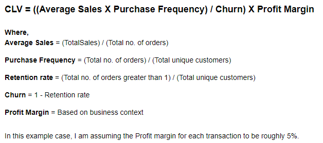
Now let’s look at the general formula for calculating the Customer Lifetime Value:
But some great analytical minds have already worked hard for us and created some frameworks/models to handle such complexity with ease.
In general, there are two broad approaches to modeling the CLV problem:
Historical Approach:
- Aggregate Model — calculating the CLV by using the average revenue per customer based on past transactions. This method gives us a single value for the CLV.
- Cohort Model — grouping the customers into different cohorts based on the transaction date, etc., and calculate the average revenue per cohort. This method gives CLV value for each cohort.
Predictive Approach:
- Machine Learning Model — using regression techniques to fit on past data to predict the CLV.
- Probabilistic Model — it tries to fit a probability distribution to the data and estimates the future count of transactions and monetary value for each transaction.
In this article, I will walk you through all the above-mentioned types except the “Machine Learning Model” (which, by the way, is modeling the CLV as a normal regression/classification modeling problem).
This is going to be a long article, so brace yourselves up and get ready. But, I can assure you that after reading this article, you will have a good understanding of the topic and various approaches to calculate Customer Lifetime Value.
Dataset Information
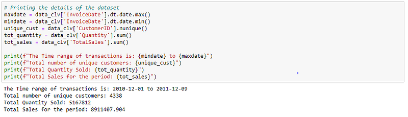
In this case study, we are going to work with the online-retail dataset from the UCI Machine Learning repository.
This is a transactional data set that contains all the transactions occurring between 01/12/2010 and 09/12/2011 for a UK-based and registered non-store online retail. The company mainly sells unique all-occasion gifts. Many customers of the company are wholesalers.
Attribute Information:
- InvoiceNo: Invoice number. Nominal, a 6-digit integral number uniquely assigned to each transaction. If this code starts with letter ‘c’, it indicates a cancellation.
- StockCode: Product (item) code. Nominal, a 5-digit integral number uniquely assigned to each distinct product.
- Description: Product (item) name. Nominal.
- Quantity: The quantities of each product (item) per transaction. Numeric.
- InvoiceDate: Invoice Date and time. Numeric, the day and time when each transaction was generated.
- UnitPrice: Unit price. Numeric, Product price per unit in sterling.
- CustomerID: Customer number. Nominal, a 5-digit integral number uniquely assigned to each customer.
- Country: Country name. Nominal, the name of the country where each customer resides.
To save some time, the complete data preprocessing step is not discussed in this article. But you can check the same along with the complete code for this article in this GitHub repository.
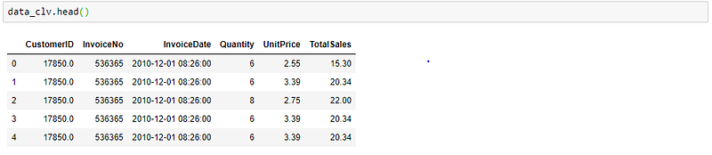
After all the preprocessing, the data will look like this:
Python Code:
Historical Approach
1. Aggregate Model:
The simplest and the oldest method of computing CLV is this Aggregate/Average method. This assumes a constant average spend and churn rate for all the customers.
This method does not differentiate between customers and produces a single value for CLV at an overall level. This leads to unrealistic estimates if some of the customers transacted in high value and high volume, which ultimately skews the average CLV value.
If you recall the formula discussed above, except Profit Margin all the other variables can be estimated/calculated. So, in this example case, I am assuming the Profit margin for each transaction to be roughly 5%.
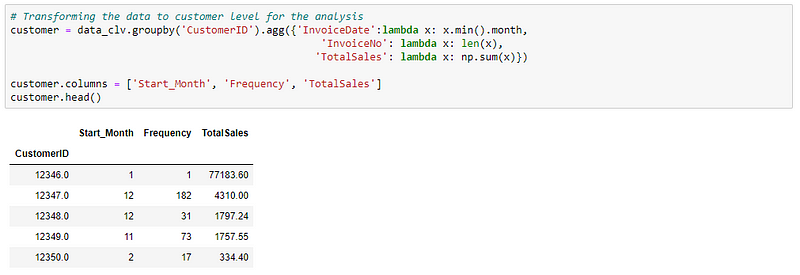
Let’s transform the data into the required format.
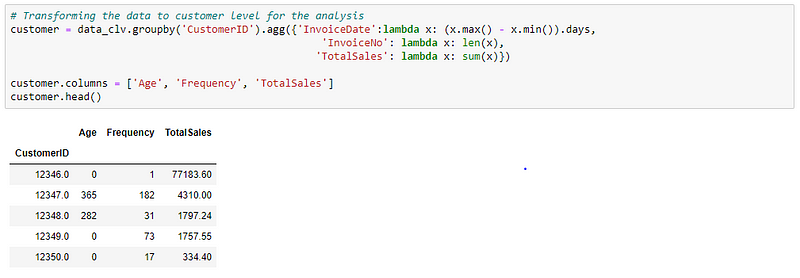
Then, calculating the variables which are to be used in the CLV formula.
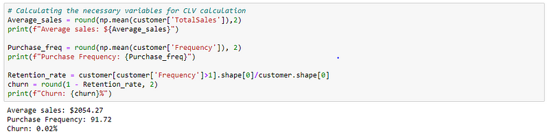
Now we have all the required variables to calculate the CLV for the Aggregate model.
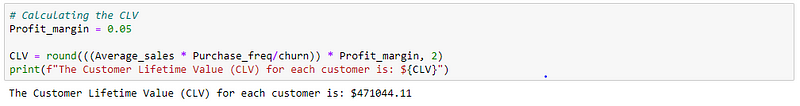
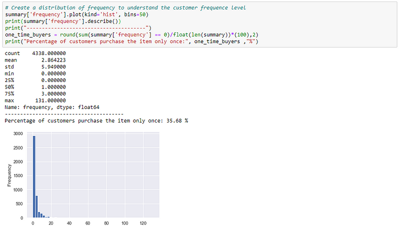
From our basic model, we got a CLV value of $471K for each customer. Do you think this number makes sense? Well, it doesn’t for me! The reason is because of the very high sales value from very few customers, which actually skewed the overall number. Also, not all customers are the same right! Take a look at it for yourself:
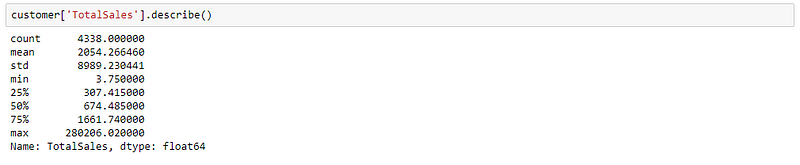
From the descriptive statistics, it is clear that almost 75% of customers in our data have a sales value of less than $2000. Whereas, the maximum sales value is around $280k. If you now look at the CLV value, do you think all the customers who transact with the business can really purchase over $470K in their lifetime? Definitely not! It varies for each customer or at least for each customer segment. This is another limitation of this model.
2. Cohort Model:
Instead of simply assuming all the customers to be one group, we can try to split them into multiple groups and calculate the CLV for each group. This model overcomes the major drawback of the simple Aggregate model which assumes the entire customers as a single group. This is called the Cohort model.
The main assumption of this model is that customers within a cohort spend similarly or in general behave similarly.
So, the question would be- “how do we group the customers?”
The most common way to group customers into cohorts is by the start date of a customer, typically by month. The best choice will depend on the customer acquisition rate, seasonality of the business, and whether additional customer information can be used.
In this case, I am grouping them into different cohorts by their start month. So, I will get 12 cohorts of customers (Jan-Dec).
First, let’s transform the data.
Then calculate CLV for each cohort.
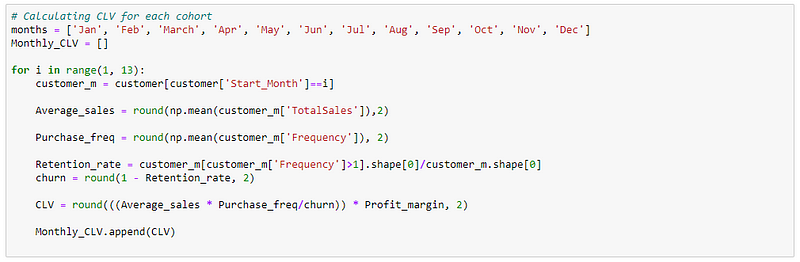
And this is the final CLV value for customers falling under each of these Monthly cohorts.
Now if you look at the result, we have 12 different CLV value for 12 months from Jan-Dec. And customers who are acquired in different months have different CLV values attached to them. This is because, they could be acquired using different campaigns, etc., so their behavior might be different from others.
Also, if you look at the values for January and December, the CLV values are quite high. This could be a false value because the data we are using is from an online retail store that sells gifts to wholesalers/companies and the festivals like Christmas, New year falls on those months. That’s why we are seeing a high CLV value for those customers who are started in January and December.
Predictive Approach
1. Probabilistic Model:
This class of models tries to fit a probability distribution to the data and then use that information to estimate other parameters of the CLV equation (such as the number of future transactions, future monetary value, etc.).
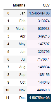
There are various probabilistic models out there that can be used to predict future CLV. One important thing to note here is that not all the variables in the CLV equation can be predicted using a single model. Usually, Transaction variables (Purchase freq & Churn) and Monetary variables (Avg order value) are modeled separately. Below is the list of probabilistic models available for the same.
In this case study, we are going to use the BG/NBD model for Transaction variables and the Gamma-Gamma model for Monetary variables.
BG/NBD stands for Beta Geometric/Negative Binomial Distribution.
This is one of the most commonly used probabilistic models for predicting the CLV. This is an alternative to the Pareto/NBD model, which is also one of the most used methods in CLV calculations. For the sake of this case, we are going to focus only on the BG/NBD model, but the steps are similar if you want to try it for Pareto/NBD.
To be specific, both the BG/NBD and Pareto/NBD model actually tries to predict the future transactions of each customer. It is then combined with the Gamma-Gamma model, which adds the monetary aspect of the customer transaction and we finally get the customer lifetime value (CLV).
The BG/NBD model has few assumptions:
1. When a user is active, number of transactions in a time t is described by Poisson distribution with rate lambda.
2. Heterogeneity in transaction across users (difference in purchasing behavior across users) has Gamma distribution with shape parameter r and scale parameter a.
3. Users may become inactive after any transaction with probability p and their dropout point is distributed between purchases with Geometric distribution.
4. Heterogeneity in dropout probability has Beta distribution with the two shape parameters alpha and beta.
5. Transaction rate and dropout probability vary independently across users.
These are some of the assumptions this model considers for predicting the future transactions of a customer.
The model fits the distribution to the historic data and learn the distribution parameter and then use them to predict future transactions of a customer.
We don’t need to worry about carrying out this complex probabilistic model by ourselves. There is a Python package called Lifetimes which makes our life easier. This package is primarily built to aid customer lifetime value calculations, predicting customer churn, etc. It has all the major models and utility functions that are needed for CLV calculations.
In this case, we are going to use just that. Let’s jump into the coding.

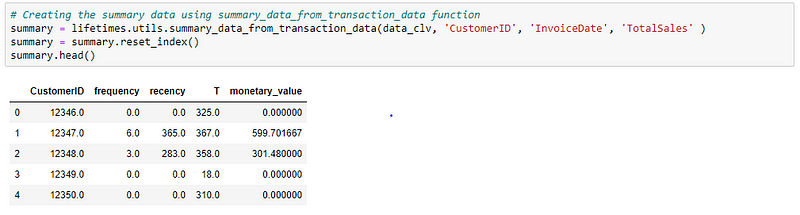
First, we need to create a summary table from the transaction data. The summary table is nothing but an RFM table. (RFM — Recency, Frequency and Monetary value)
For this, we can use the summary_data_from_transactions_data function in the Lifetimes package. What it does is, it aggregates the transaction-level data into the customer level and calculates the frequency, recency, T, and monetary_value for each customer.
- frequency — the number of repeat purchases (more than 1 purchases)
- recency — the time between the first and the last transaction
- T — the time between the first purchase and the end of the transaction period (last date of the time frame considered for the analysis)
- monetary_value — it is the mean of a given customers sales value
Here the value of 0 in frequency and recency means that these are one-time buyers. Let’s check how many such one time buyers are there in our data.
Now, let’s fit the BG/NBD model to our summary data.
BG/NBD model is available as BetaGeoFitter class in Lifetimes package.
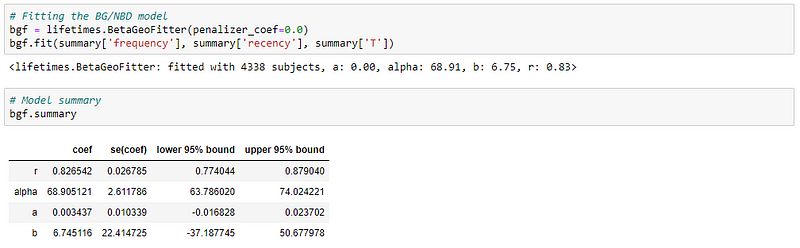
The above table shows the estimated distribution parameter values from the historical data. The model now uses this to predict future transactions and the customer churn rate.
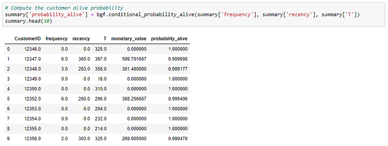
So, let’s say you want to know whether a customer is now alive or not (or predict customer churn) based on the historical data. The lifetime package provides a way to accomplish that task. You can use:
- model.conditional_probability_alive(): This method computes the probability that a customer with history (frequency, recency, T) is currently alive.
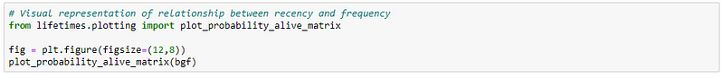
- plot_probabilty_alive_matrix(model): This function from lifetimes.plotting will help to visually analyze the relationship between recency & frequency and the customer being alive.
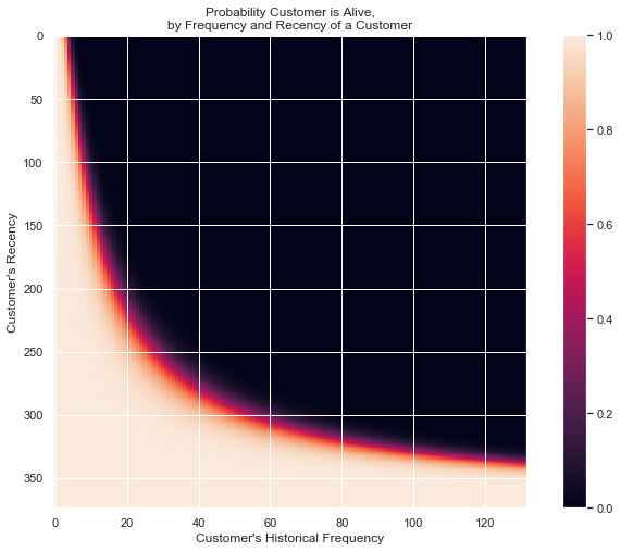
Let me explain the above two results.
The probability of being alive is calculated based on the recency and frequency of a customer. So,
- If a customer has bought multiple times (frequency) and the time between the first & last transaction is high (recency), then his/her probability of being alive is high.
- Similarly, if a customer has less frequency (bought once or twice) and the time between first & last transaction is low (recency), then his/her probability of being alive is high.
The next thing we can do with this trained model is to predict the likely future transactions for each customer. You can use:
- model.conditional_expected_number_of_purchases_up_to_time(): Calculate the expected number of repeat purchases up to time t for a randomly chosen individual from the population (or the whole population), given they have purchase history (frequency, recency, T).
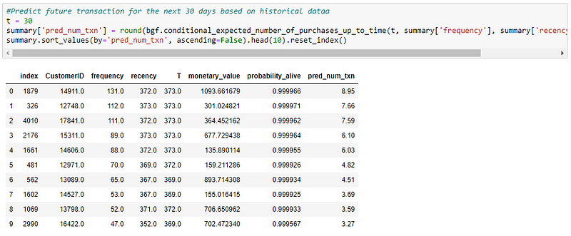
We now have the prediction for the number of purchases a customer will make in the next 10 days.
To check whether the predicted number makes sense, we can try something like this:
Let’s take CustomerID — 14911,
In 372 days, he purchased 131 times. So, in one day he purchases 131/372 = 0.352 times. Hence, for 10 days = 3.52 times.
Here, our predicted result is 8.95, which is reasonably closer to the manual probability prediction we did above. The reason for the difference is caused by the various assumptions about the customers, such as the dropout rate, customer lifetime being modeled as exponential distribution, etc.
Now that we predicted the expected future transactions, we now need to predict the future monetary value of each transaction.
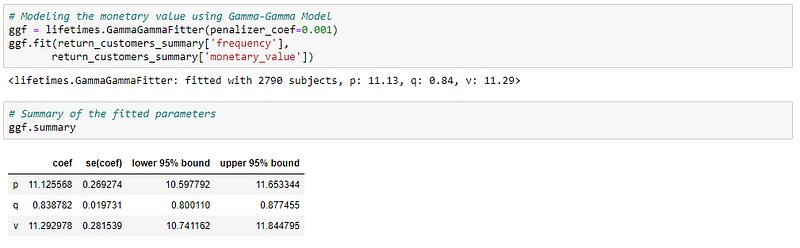
Like I have previously mentioned above, the BG/NBD model can only be able to predict the future transactions and churn rate of a customer. To add the monetary aspect of the problem, we have to model the monetary value using the Gamma-Gamma Model.
Some of the key assumptions of the Gamma-Gamma model are:
1. The monetary value of a customer’s given transaction varies randomly around their average transaction value.
2. Average transaction value varies across customers but do not vary over time for any given customer.
3. The distribution of average transaction values across customers is independent of the transaction process.
As a first step before fitting the model to the data, we have to check whether the assumptions made by the model holds good for the data. Only if it satisfies, we have to proceed further.
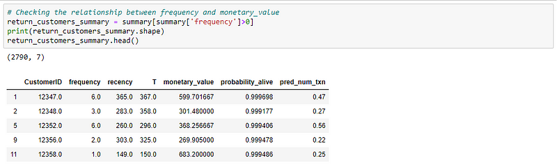
Out of the three, the final assumption can be validated. What it means is that there should not be any relationship between the frequency and monetary value of transactions. This can be easily validated using the Pearson correlation.
NOTE: We are considering only customers who made repeat purchases with the business i.e., frequency > 0. Because, if the frequency is 0, it means that they are a one-time customer and are considered already dead.
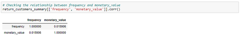
The correlation seems very weak. Hence, we can conclude that the assumption is satisfied and we can fit the model to our data.
Next, we can predict the expected average profit for each transaction and Customer Lifetime Value using the model.
- model.conditional_expected_average_profit(): This method computes the conditional expectation of the average profit per transaction for a group of one or more customers.
- model.customer_lifetime_value(): This method computes the average lifetime value of a group of one or more customers. This method takes in the BG/NBD model and the prediction horizon as a parameter to calculate the CLV.
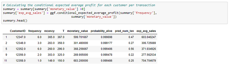
NOTE: The reason why I have mentioned as expected average sales is that the monetary value we are using is actual sales value, not the profit. Using the above method, we will get the average sales and finally, we can multiply the result by our profit margin to arrive at the actual profit value.
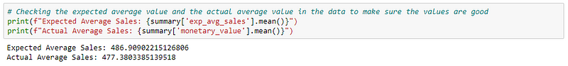
The values seem to be fine. Now, let’s calculate the customer lifetime value directly using the method from the lifetime’s package.
Three main important things to note here is:
- time: This parameter in the customer_lifetime_value() method takes in terms of months i.e., t=1 means one month, and so on.
- freq: This parameter is where you will specify the time unit your data is in. If your data is on a daily level then “D”, monthly “M” and so on.
- discount_rate: This parameter is based on the concept of DCF (discounted cash flow), where you will discount the future monetary value by a discount rate to get the present value of that cash flow. In the documentation, it is given that for monthly it is 0.01 (annually ~12.7%).
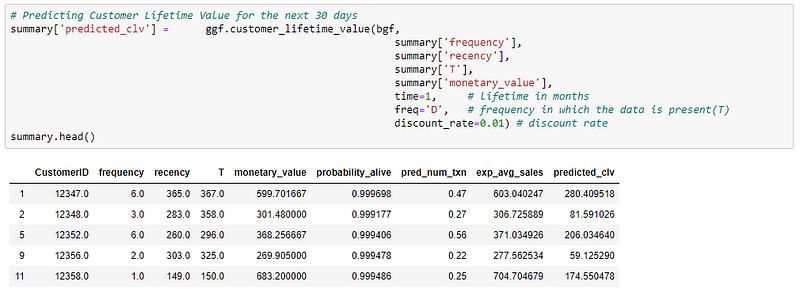
You can also calculate the CLV manually from the predicted number of future transactions (pred_num_txn) and expected average sales per transaction (exp_avg_sales).

Both the CLV values are very close to each other and seem reasonable for the next 30 days.
One thing to note here is that, both the values we have calculated for CLV is the sales value, not the actual profit. To get the net profit for each customer, we can either create profit value in the beginning by multiplying sales value with profit margin or we can do that now.
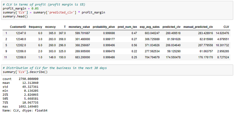
Finally, we predicted the CLV for each customer for the next 30 days.
The marketing team can now use this information to target customers and increase their sales.
Also, it is hard to target each customer. If we have access to customer demographics data, we can first create customer segmentation and then predict the CLV value for each segment. This segment level information can then be used for personalized targeting. If there is no access/availability of customer demographics data, then an easy way would be to use RFM segmentation and then predict CLV for those RFM segments.
I hope this helps you understand the concept behind Customer Lifetime Value calculation and different ways to calculate it.


Comprehensive article with detailed approach on CLV as a whole :)
This is really good and comprehensive. Thanks Hari for sharing :)
First of all, I want to appreciate the detailed explanation on CLV. I am addressing my question for this approach. In the table containing alive_probability, why the probability for customer 12346 is 1 as this person had 0 frequency and recency which should be treated as churned? Moreover, should a one-time transaction always be treated as churned? What if the customer just enrolled and paid 1 day before the last date of the this analysis, i.e, T = 1? Finally, when training the BG/NBD model, should the rows of the one-time purchase customer removed from the model as these records were treated as churned already?
Hi Hari, Thank you for such a detailed explanation.. great work!! I have a question regarding probabilistic approach models. My data has RFM features but they are grouped in different buckets (ex: Recency - (1(new)-4(old), same way for frequency and monetary value)). Can I run the BG/NBD and gamma gamma on this data directly?
Great article! One quick question is can we use the profit value in the calculation instead of the actual monetary value? For example, suppose we have a different profit margin per item or customer and would like to integrate it into the prediction.
Very nicely put informative article . Helpful. Note: while showing the calculation of future transactions, code calculates 30 days while the explanation calculates for 10 days. It is a little confusing.
Great article! Quick question. In the historical approach, for your average_sales, you take the mean of the customer['totalSales']. But that would just average over the number of customers. Wouldn't you instead want the average over all orders, i.e., customer['totalSales'].sum()/customer['frequency'].sum()?
Customer alive probability based on recency (this article definition) and frequency are completely wrong. 1. Customer who made a single purchase 5 years ago 2. Customer who just made a purchase in both cases, frequency and recency will be 0 and alive probability is 1 where we all know for 1st case alive probability will be close to 0
Good article. One problem: summary = lifetimes.utils.summary_data_from_transaction_data(data_clv, 'CustomerID', 'InvoiceDate', 'TotalSales') can produce negative values for monetary_value, which in turn later on causes: ggf.fit(return_customers_summary['frequency'], return_customers_summary['monetary_value']) to blow up if they aren't first excluded.