All About Decision Tree from Scratch with Python Implementation
Introduction
If you see, you will find out that today, ensemble learnings are more popular and used by industry and rankers on Kaggle. Bootstrap aggregation, Random forest, gradient boosting, XGboost are all very important and widely used algorithms, to understand them in detail one needs to know the decision tree in depth. In this article, we are going to cover just that. Without any further due, let’s just dive right into it.
Table of Content
- Introduction to decision tree
- Types of Decision Tree
- How to Build a decision Tree from data
- Avoid over-fitting in decision trees
- Advantages and disadvantages of Decision Tree
- Implementing a decision tree using Python
Introduction to Decision Tree
Formally a decision tree is a graphical representation of all possible solutions to a decision. These days, tree-based algorithms are the most commonly used algorithms in the case of supervised learning scenarios. They are easier to interpret and visualize with great adaptability. We can use tree-based algorithms for both regression and classification problems, However, most of the time they are used for classification problem.
Let’s understand a decision tree from an example: Yesterday evening, I skipped dinner at my usual time because I was busy taking care of some stuff. Later in the night, I felt butterflies in my stomach. I thought only if I wasn’t hungry, I could have gone to sleep as it is but as that was not the case, I decided to eat something. I had two options, to order something from outside or cook myself.
I figured if I order, I will have to spare at least INR 250 on it. I finally decided to order it anyway as it was pretty late and I was in no mood of cooking. This complete incident can be graphically represented as shown in the following figure.
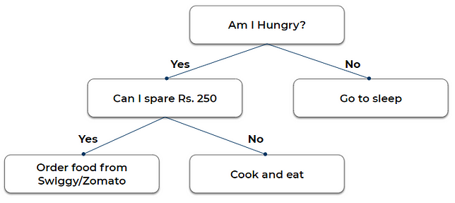
This representation is nothing but a decision tree.
Terminologies associated with decision tree
- Parent node: In any two connected nodes, the one which is higher hierarchically, is a parent node.
- Child node: In any two connected nodes, the one which is lower hierarchically, is a child node.
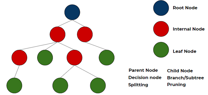
- Root node: The starting node from which the tree starts, It has only child nodes. The root node does not have a parent node. (dark blue node in the above image)
- Leaf Node/leaf: Nodes at the end of the tree, which do not have any children are leaf nodes or called simply leaf. (green nodes in the above image)
- Internal nodes/nodes: All the in-between the root node and the leaf nodes are internal nodes or simply called nodes. internal nodes have both a parent and at least one child. (red nodes in the above image)
- Splitting: Dividing a node into two or more sun-nodes or adding two or more children to a node.
- Decision node: when a parent splits into two or more children nodes then that node is called a decision node.
- Pruning: When we remove the sub-node of a decision node, it is called pruning. You can understand it as the opposite process of splitting.
- Branch/Sub-tree: a subsection of the entire tree is called a branch or sub-tree.
Types of Decision Tree
Regression Tree
A regression tree is used when the dependent variable is continuous. The value obtained by leaf nodes in the training data is the mean response of observation falling in that region. Thus, if an unseen data observation falls in that region, its prediction is made with the mean value. This means that even if the dependent variable in training data was continuous, it will only take discrete values in the test set. A regression tree follows a top-down greedy approach.
Classification Tree
A classification tree is used when the dependent variable is categorical. The value obtained by leaf nodes in the training data is the mode response of observation falling in that region It follows a top-down greedy approach.
Together they are called as CART(classification and regression tree)
Building a decision Tree from data
How to create a tree from tabular data? which feature should be selected as the root node? on what basis should a node be split? To all these questions answer is in this section
The decision of making strategic splits heavily affects a tree’s accuracy. The purity of the node should increase with respect to the target variable after each split. The decision tree splits the nodes on all available variables and then selects the split which results in the most homogeneous sub-nodes.
The following are the most commonly used algorithms for splitting
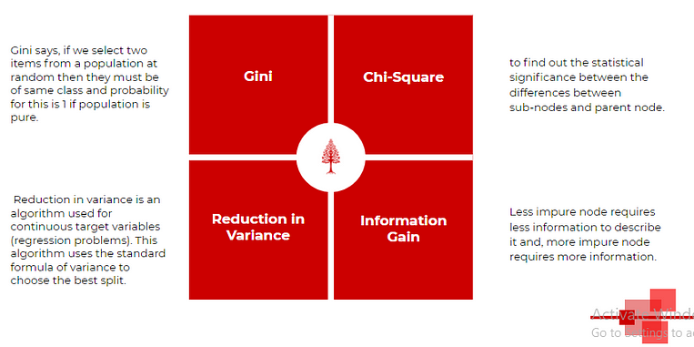
1. Gini impurity
Gini says, if we select two items from a population at random then they must be of the same class and the probability for this is 1 if the population is pure.
- It works with the categorical target variable “Success” or “Failure”.
- It performs only Binary splits
- Higher the value of Gini higher the homogeneity.
- CART (Classification and Regression Tree) uses the Gini method to create binary splits.
Steps to Calculate Gini impurity for a split
- Calculate Gini impurity for sub-nodes, using the formula subtracting the sum of the square of probability for success and failure from one.
1-(p²+q²)
where p =P(Success) & q=P(Failure) - Calculate Gini for split using the weighted Gini score of each node of that split
- Select the feature with the least Gini impurity for the split.
2. Chi-Square
It is an algorithm to find out the statistical significance between the differences between sub-nodes and parent node. We measure it by the sum of squares of standardized differences between observed and expected frequencies of the target variable.
- It works with the categorical target variable “Success” or “Failure”.
- It can perform two or more splits.
- Higher the value of Chi-Square higher the statistical significance of differences between sub-node and Parent node.
- Chi-Square of each node is calculated using the formula,
- Chi-square = ((Actual — Expected)² / Expected)¹/2
- It generates a tree called CHAID (Chi-square Automatic Interaction Detector)
Steps to Calculate Chi-square for a split:
- Calculate Chi-square for an individual node by calculating the deviation for Success and Failure both
- Calculated Chi-square of Split using Sum of all Chi-square of success and Failure of each node of the split
- Select the split where Chi-Square is maximum.
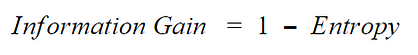
3. Information Gain
A less impure node requires less information to describe it and, a more impure node requires more information. Information theory is a measure to define this degree of disorganization in a system known as Entropy. If the sample is completely homogeneous, then the entropy is zero and if the sample is equally divided (50% — 50%), it has an entropy of one. Entropy is calculated as follows.
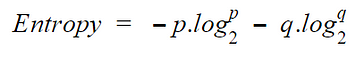
Steps to calculate entropy for a split:
- Calculate the entropy of the parent node
- Calculate entropy of each individual node of split and calculate the weighted average of all sub-nodes available in the split. The lesser the entropy, the better it is.
- calculate information gain as follows and chose the node with the highest information gain for splitting
4. Reduction in Variance
Till now, we have discussed the algorithms for the categorical target variable. Reduction in variance is an algorithm used for continuous target variables (regression problems).
- Used for continuous variables
- This algorithm uses the standard formula of variance to choose the best split.
- The split with lower variance is selected as the criteria to split the population
Steps to calculate Variance:
- Calculate variance for each node.

- Calculate variance for each split as a weighted average of each node variance.
- The node with lower variance is selected as the criteria to split.
In summary:
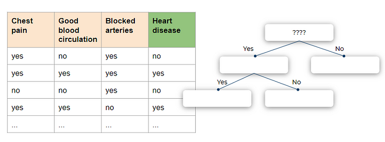
In practice, most of the time Gini impurity is used as it gives good results for splitting and its computation is inexpensive. Let’s build a tree with a pen and paper. We have a dummy dataset below, the features(X) are Chest pain, Good blood circulation, Blocked arteries and to be predicted column is Heart disease(y). Every column has two possible options yes and no.
We aim to build a decision tree where given a new record of chest pain, good blood circulation, and blocked arteries we should be able to tell if that person has heart disease or not. At the start, all our samples are in the root node. We will have to decide on which of the feature the root node should be divided first.
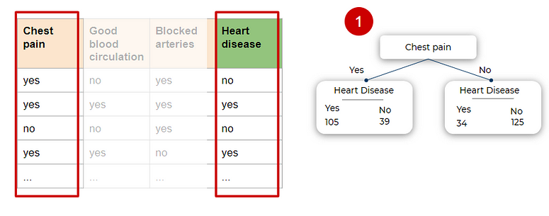
We will focus first on how heart disease is changing with Chest pain (ignoring good blood circulation and blood arteries). the dummy numbers are shown below
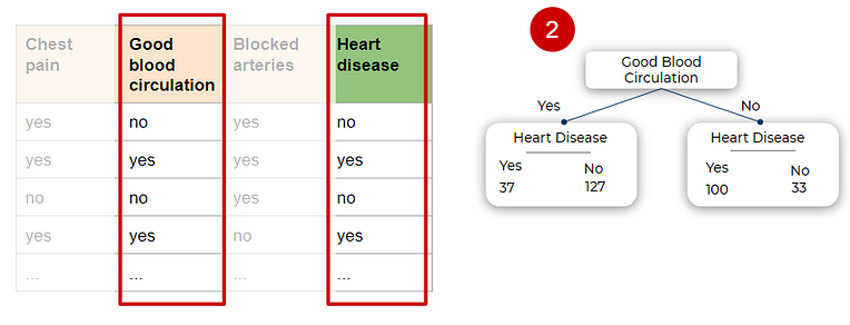
Similarly, we divide based on good communication as shown in the below image.
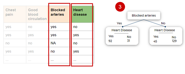
And with respect to blocked arteries as below image.
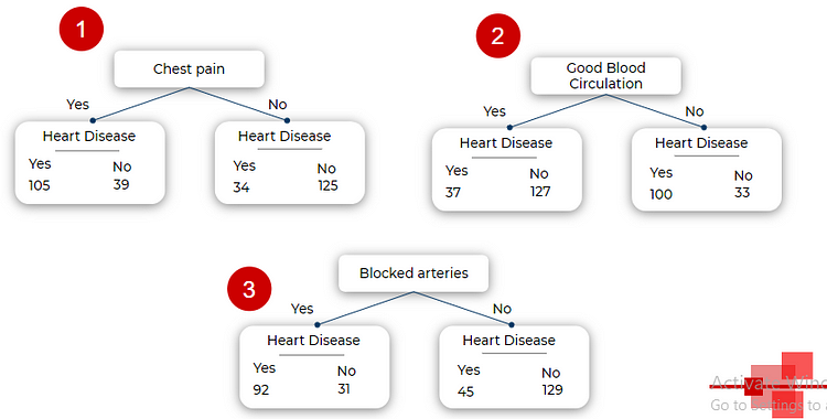
Taking all three splits at one place in the below image. We can observe that, it is not a great split on any of the feature alone for heart disease yes or no which means that one of these can be a root node but its not a full tree, we will have to split again down the tree in hope of better split.
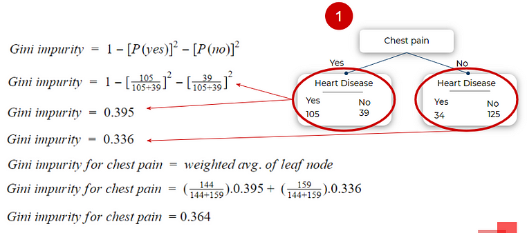
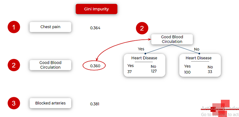
To decide on which one feature should the root node be split, we need to calculate the Gini impurity for all the leaf nodes as shown below. After calculating for leaf nodes, we take its weighted average to get Gini impurity about the parent node.
We do this for all three features and select the one with the least Gini impurity as it is splitting the dataset in the best way out of three. Hence we choose good blood circulation as the root node.
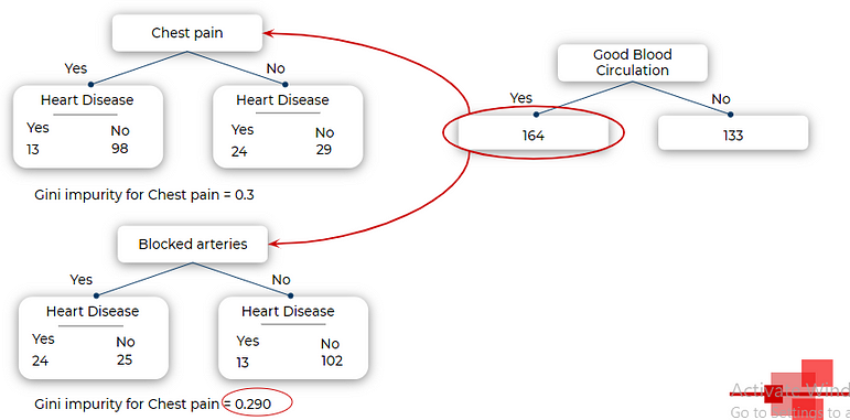
We do the same for a child node of Good blood circulation now. In the below image we will split the left child with a total of 164 sample on basis of blocked arteries as its Gini impurity is lesser than chest pain(we calculate Gini index again with the same formula as above, just a smaller subset of the sample — 164 in this case).
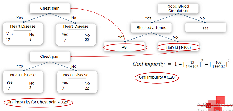
One thing to note in the below image that, when we try to split the right child of blocked arteries on basis of chest pain, the Gini index is 0.29 but the Gini impurity of the right child of the blocked tree itself, is 0.20. This means that splitting this node any further is not improving impurity. so this will be a leaf node.
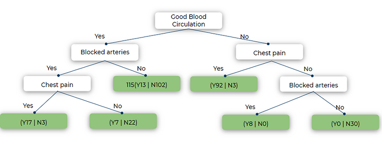
We repeat the same process for all the nodes and we get the following tree. This looks a good enough fit for our training data.
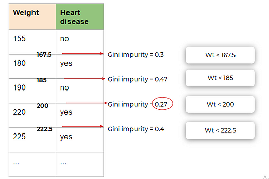
This is how we create a tree from data. What should we do if we have a column with numerical values? It is simple, order them in ascending order. Calculate the mean on every two consecutive numbers. make a split on basis of that and calculate Gini impurity using the same method. We choose the split with the least Gini impurity as always.
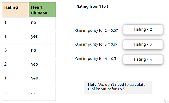
If we have ranked the numerical column in the dataset, we split on every rating and calculate Gini impurity for each split, and select the one with the least Gini impurity.
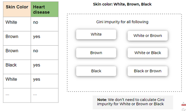
If we have categorical choices in our dataset then the split and Gini impurity calculation needs to be done on every possible combination of choices
Avoid Overfitting in Decision Trees
Overfitting is one of the key challenges in a tree-based algorithm. If no limit is set, it will give 100% fitting, because, in the worst-case scenario, it will end up making a leaf node for each observation. Hence we need to take some precautions to avoid overfitting. It is mostly done in two ways:
- Setting constraints on tree size
- Tree pruning
Let’s discuss both of these briefly.
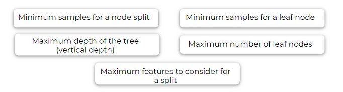
Setting Constraints on tree size
Parameters play an important role in tree modeling. Overfitting can be avoided by using various parameters that are used to define a tree.
- Minimum samples for a node split
- Defines the minimum number of observations that are required in a node to be considered for splitting. (this ensures above mentioned worst-case scenario).
- A higher value of this parameter prevents a model from learning relations that might be highly specific to the particular sample selected for a tree.
- Too high values can lead to under-fitting hence, it should be tuned properly using cross-validation.
-
Minimum samples for a leaf node
- Defines the minimum observations required in a leaf. (Again this also prevents worst-case scenarios)
- Generally, lower values should be chosen for imbalanced class problems as the regions in which the minority class will be in majority will be of small size.
- Maximum depth of the tree (vertical depth)
- Used to control over-fitting as higher depth will allow the model to learn relations very specific to a particular sample.
- Should be tuned properly using Cross-validation as too little height can cause underfitting.
- Maximum number of leaf nodes
- The maximum number of leaf nodes or leaves in a tree.
- Can be defined in place of max_depth. Since binary trees are created, a depth of
nwould produce a maximum of2^nleaves.
-
Maximum features to consider for a split
- The number of features to consider while searching for the best split. These will be randomly selected.
- As a thumb-rule, the square root of the total number of features works great but we should check up to 30–40% of the total number of features.
- Higher values can lead to over-fitting but depend on case to case.
Pruning
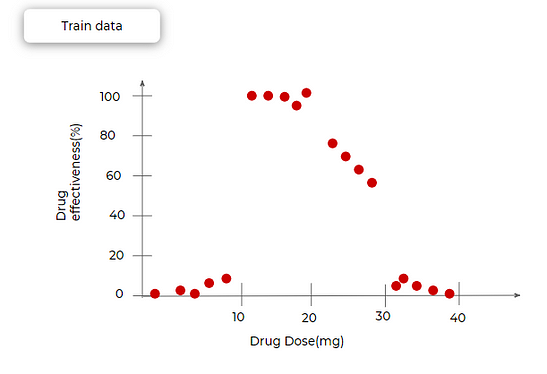
Recall from terminologies, pruning is something opposite to splitting. Now we see how exactly that is the case. Let’s see the following example where drug effectiveness is plotted against drug doses. All the red points are the training dataset. We can see that for very small and very large quantities of doses, the drug effectiveness is almost negligible. Between 10–20mg, almost 100% and gradually decreasing between 20 to 30.
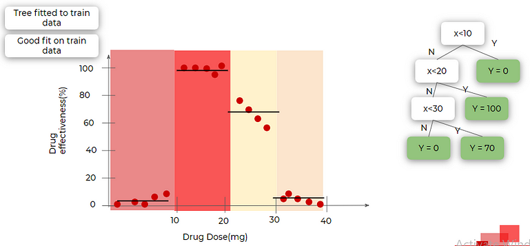
We modeled a tree and we got the following results. we did splitting at three places and got 4 leaf nodes which will give output as 0(y): 0–10(X), 100:10–20, 70:20–30, 0:30–40 respectively as we increase the doses. It is a great fit for the training dataset, the black horizontal lines are output given for the node.
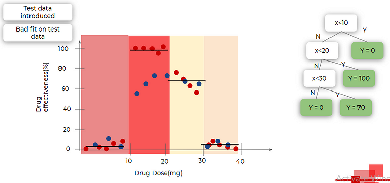
Let’s test it on the training dataset (blue dots in the following image are of the testing dataset). It is a bad fit for testing data. A good fit for training data and a bad fit for testing data means overfitting.
To overcome the overfitting issue of our tree, we decide to merge two segments in the middle which means removing two nodes from the tree as you can see in the image below(the nodes with the red cross on them are removed). now again we fit this tree on the training dataset. Now, the tree is not that great fit for training data.
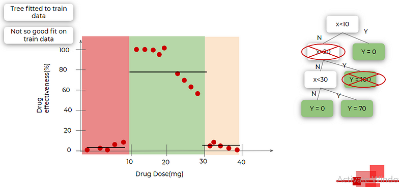
But, when we introduce testing data, it performs better than before.
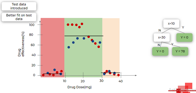
This is basically pruning. Using pruning we can avoid overfitting to the training dataset.
Advantages and disadvantages of Decision Tree
Advantages of a decision tree
- Easy to visualize and interpret: Its graphical representation is very intuitive to understand and it does not require any knowledge of statistics to interpret it.
- Useful in data exploration: We can easily identify the most significant variable and the relation between variables with a decision tree. It can help us create new variables or put some features in one bucket.
- Less data cleaning required: It is fairly immune to outliers and missing data, hence less data cleaning is needed.
- The data type is not a constraint: It can handle both categorical and numerical data.
Disadvantages of decision tree
- Overfitting: single decision tree tends to overfit the data which is solved by setting constraints on model parameters i.e. height of the tree and pruning(which we will discuss in detail later in this article)
- Not exact fit for continuous data: It losses some of the information associated with numerical variables when it classifies them into different categories.
Implementing a decision tree using Python
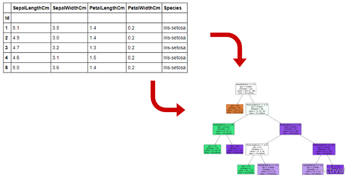
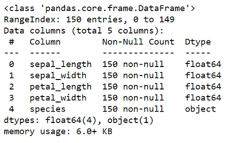
In this section, we will see how to implement a decision tree using python. We will use the famous IRIS dataset for the same. The purpose is if we feed any new data to this classifier, it should be able to predict the right class accordingly.
You can get complete code for this implementation here
Importing the Required Libraries and Reading the data
First thing is to import all the necessary libraries and classes and then load the data from the seaborn library.
Python Code:
you should be able to get the above data. Here we have 4 feature columns sepal_length, sepal_width, petal_length, and petal_width respectively with one target column species.
EDA
Now performing some basic operations on it.
#getting information of dataset
df.info()
df.shape

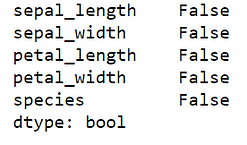
we understand that this dataset has 150 records, 5 columns with the first four of type float and last of type object str and there are no NAN values as form following command
df.isnull().any()
Now we perform some basic EDA on this dataset. Let’s check the correlation of all the features with each other
# let's plot pair plot to visualise the attributes all at once
sns.pairplot(data=df, hue = 'species')
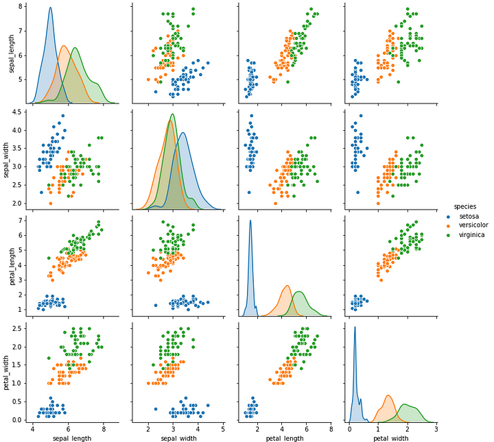
We have a total of 3 species that we want to predict: setosa, versicolor, and virginica. We can see that setosa always forms a different cluster from the other two.
# correlation matrix
sns.heatmap(df.corr())
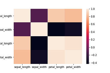
We can observe from the above two plots:
- Setosa always forms a different cluster.
- Petal length is highly related to petal width.
- Sepal length is not related to sepal width.
Data Preprocessing
Now, we will separate the target variable(y) and features(X) as follows
target = df['species']
df1 = df.copy()
df1 = df1.drop('species', axis =1)
It is good practice not to drop or add a new column to the original dataset. Make a copy of it and then modify it so in case things don’t work out as we expected, we have the original data to start again with a different approach.
Just for the sake of following mostly used convention, we are storing df in X
# Defining the attributes
X = df1
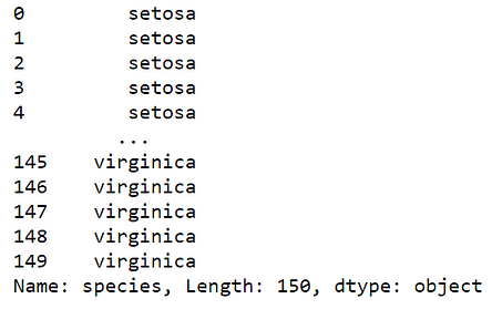
Now let’s look at our target variable
target
target has categorical variables stored in it we will encode it in numeric values for working.
#label encoding
le = LabelEncoder()
target = le.fit_transform(target)
target
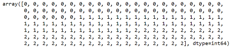
We get its encoding as above, setosa:0, versicolor:1, virginica:2
Again for the sake of following the standard naming convention, naming target as y
y = target
Splitting the dataset into training and testing sets. selecting 20% records randomly for testing
# Splitting the data - 80:20 ratio
X_train, X_test, y_train, y_test = train_test_split(X , y, test_size = 0.2, random_state = 42)print("Training split input- ", X_train.shape)
print("Testing split input- ", X_test.shape)
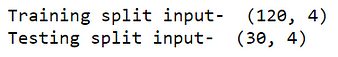
After splitting the dataset we have 120 records(rows) for training and 30 records for testing purposes.
Modeling Tree and testing it
# Defining the decision tree algorithmdtree=DecisionTreeClassifier()
dtree.fit(X_train,y_train)print('Decision Tree Classifier Created')
In the above code, we created an object of the class DecisionTreeClassifier , store its address in the variable dtree, so we can access the object using dtree. Then we fit this tree with our X_train and y_train . Finally, we print the statement Decision Tree Classifier Created after the decision tree is built.
# Predicting the values of test data
y_pred = dtree.predict(X_test)
print("Classification report - \n", classification_report(y_test,y_pred))
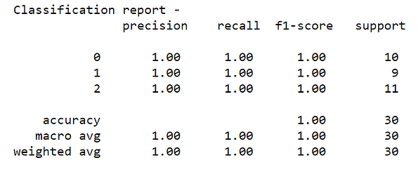
We got an accuracy of 100% on the testing dataset of 30 records.
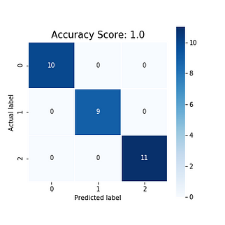
let’s plot the confusion matrix as follows
cm = confusion_matrix(y_test, y_pred)
plt.figure(figsize=(5,5))sns.heatmap(data=cm,linewidths=.5, annot=True,square = True,  cmap = 'Blues')plt.ylabel('Actual label')
plt.xlabel('Predicted label')all_sample_title = 'Accuracy Score: {0}'.format(dtree.score(X_test, y_test))
plt.title(all_sample_title, size = 15)
Visualizing the decision tree
We can directly plot the tree that we build using the following commands
# Visualising the graph without the use of graphvizplt.figure(figsize = (20,20))
dec_tree = plot_tree(decision_tree=dtree, feature_names = df1.columns,
                     class_names =["setosa", "vercicolor", "verginica"] , filled = True , precision = 4, rounded = True)
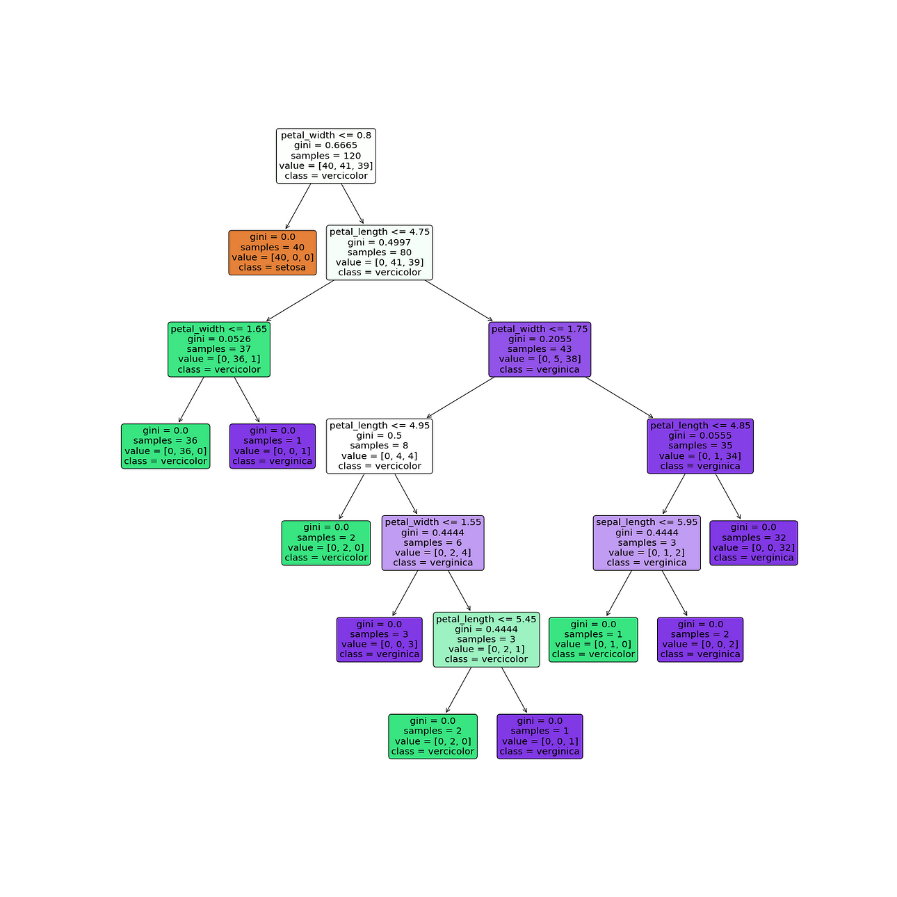
We can see how the tree is split, what are the gini for the nodes, the records in those nodes, and their labels.
All the images are from the author unless given credit explicitly.
If you want to learn the basics of visualization using seaborn or EDA you can find it here-
All the images are from the author unless given credit
About the Author

Sanket Kangle
Data Scientist, IIT KGP alumnus, knowledge and expertise in conceptualizing and scaling a business solution based on new-age technologies — AI, Cloud


Awesome explanation
Using Python in jupyter notebook how to plot the decision tree.it would be good ilif you would have gone step by step.getting confused between your explanation and my teacher class.