Generate Background Blur using Deep Learning in Python with this Simple Tutorial
Overview
- Get to know the deep learning model we will use and ReLu6
- Understand how to get blur background using deep learning
Introduction
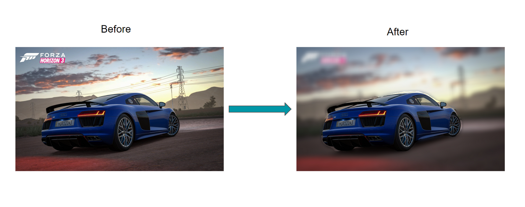
The background blur effect which is also known as “bokeh” is a well-known effect that is used by many of us mainly for close up shots. It adds a sense of depth to our image as we only concentrate on a particular part of our image.
To get this kind of effect we generally use some photo editing applications like Photoshop, Gimp, Picsart, Snapseed, etc. As time progressed we made significant improvements in terms of computer vision and image processing using deep learning. So there arises a question can we get this bokeh effect using deep learning? The answer is – yes! we can. In the following blog, I will walk you through the complete implementation along with the code and some theoretical aspects for better understanding.
Contents
- How it is achieved?
- Deep Learning model that we will be using
- ReLu6
- Implementation
- Credits
- Conclusion
1. How it is achieved?
Basically the whole objective is based on the advance implementation of a convolution neural network called image segmentation. We all are familiar with CNN’s which are used for the classification of images, based on the number of input labels we have. But suppose we have to identify a particular object in a given image for this we have to use the concept of object detection and then image segmentation.

Source-Google
This is the classic example of image classification and detection where if there are multiple classes of the object are available in a single image then we go for object detection, the given image goes undergoes region of interest pooling once we find the coordinates of multiple objects in an image after that these objects are classified and bounding boxes are drawn around every identified object.
Once all this is done then we proceed to the next step of segmentation of image because the bounding boxes only show where the object is located inside the image but it does not give any information about the shape of the object.
In simple terms, image segmentation is the process of dividing the image pixels into small parts or segments and group them based on similar information or attributes, and assigning them a label. This helps to capture very small details on the pixel level. Segmentation creates a pixel-wise mask for every identified object in the image, please have a look at the picture below. The main aim is to train the neural network in such a way that it can give a pixel-wise mask of the image. To understand this in more detail then click here.

Source – MissingLink.ai
2. The deep learning model that we will be using:
Once we are clear with image segmentation, then let’s have a look at the model that we will be using, i.e. the mobilenetv2 which is trained on the coco dataset.
The mobilenetv2 is a lightweight model that can be used on low powered devices like mobile phones, this is the second version of the mobilenetv1 model which came out in 2017.
Now let us briefly understand the model architecture.
Source- towardsdatascience
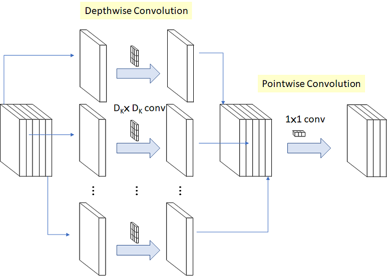
The v2 is also based on v1 so it inherits the same depth-wise separable convolution which consists of depthwise convolution and pointwise convolution which reduces the cost of the convolution operation.
The depth-wise convolution simply means that suppose an image contains 3 channels then each kernel will iterate over each channel respectively.
For example, you have an image of (10 x 10 x 3) and 3 filters of (3 x 3 x 1) then the resultant output will be (8 x 8 x 1) of one such filter after which outputs of all the other filters are stacked up together and forming feature map consisting of (8 x 8 x 3).
In pointwise convolution, we take the previous feature map of (8 x 8 x 3) and apply a filter of size (1 x 1 x 3). If 15 such filters are applied then the final result will be stacked up to form a feature map of (8 x 8 x 15).
The mobilenetv2 has some improvements over v1 like the implementation of inverted residuals, linear bottlenecks, and the residual connection.

Source-MachineThink.Net
The v2 comes total with 3 convolution layers, in which the first one is the expansion layer, the second one is the depth-wise layer, and the third one is the projection layer.
Expansion Layer: this layer takes the input data and expands the lower dimension data into higher dimensions so that the important information is preserved and gives its output to the depth-wise layer, the factor of expansion is a hyperparameter which can be tuned depending upon the number of trials.
Depth-wise Layer: this layer receives the input from the expansion layer and performs the depth-wise and pointwise convolution, gives the feature map to the projection layer.
Projection Layer: this layer is responsible to shrink down the dimension of data so that only a limited amount of the data is passed further in the network, at this point in time the input dimension matches the output dimension and it is also known as “bottleneck layer”.

Source-MachineThink.Net
The residual connection is a new addition to the network, which is based on the ResNet and helps to control the flow of gradients through the network. It is used when the dimension of input data is the same as the output data.
3. ReLu6:
Source-Google
Each layer in this network comes with ReLu6 rather than ReLu along with Batch Normalization. The ReLu6 limits the range of values between 0 to 6, which is a linear activation function. It also helps to hold precision to the right of the decimal point by limiting 3 bits of information to the left of the decimal point.
The output of the last layer i.e. projection layer does not have an activation function as its output is a low dimension data, according to the researchers adding any non-linear function to the last layer may cause loss of useful information.
4. Implementation
Now as we have a brief idea about image segmentation and the mobilenetv2 which we will be using let’s go with the implementation part.
Prerequisite:- the code uses TensorFlow version 1.x so you need to have version 1.x for it to work, if you are using 2.x then it will get errors while executing so I would suggest simply use Google Collab for executing it.
I will be going through a quick walkthrough of all the important aspects of code and the complete implementation with a line-by-line explanation in my notebook on GitHub.
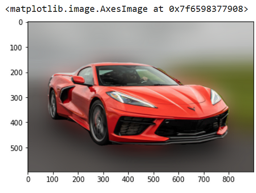
For demonstration, we will be using the below image of size (596 x 900)

Step 1: Downloading the pre-trained model.
As the model is pre-trained only need to download it and pass our image to it, and it will return the segmented image.
MODEL_NAME = 'mobilenetv2_coco_voctrainaug'  # @param ['mobilenetv2_coco_voctrainaug', 'mobilenetv2_coco_voctrainval', 'xception_coco_voctrainaug', 'xception_coco_voctrainval']_DOWNLOAD_URL_PREFIX = 'http://download.tensorflow.org/models/'
_MODEL_URLS = {
    'mobilenetv2_coco_voctrainaug':
        'deeplabv3_mnv2_pascal_train_aug_2018_01_29.tar.gz',
    'mobilenetv2_coco_voctrainval':
        'deeplabv3_mnv2_pascal_trainval_2018_01_29.tar.gz',
    'xception_coco_voctrainaug':
        'deeplabv3_pascal_train_aug_2018_01_04.tar.gz',
    'xception_coco_voctrainval':
        'deeplabv3_pascal_trainval_2018_01_04.tar.gz',
}
_TARBALL_NAME = 'deeplab_model.tar.gz'model_dir = tempfile.mkdtemp()
tf.gfile.MakeDirs(model_dir)download_path = os.path.join(model_dir, _TARBALL_NAME)
print('downloading model, this might take a while...')
urllib.request.urlretrieve(_DOWNLOAD_URL_PREFIX + _MODEL_URLS[MODEL_NAME],
                   download_path)
print('download completed! loading DeepLab model...')MODEL = DeepLabModel(download_path)
print('model loaded successfully!')

Output
Step 2: Function for visualizing the segmented image taken from the input.
def run_visualization():
  """Inferences DeepLab model and visualizes result."""
  try:
    original_im = Image.open(IMAGE_NAME)
  except IOError:
    print('Cannot retrieve image. Please check url: ' + url)
    returnprint('running deeplab on image')
  resized_im, seg_map = MODEL.run(original_im)
  vis_segmentation(resized_im, seg_map)
  return resized_im, seg_map
2.1: Calling the above function with the image shown previously.
IMAGE_NAME = 'download2.jpg'
resized_im, seg_map = run_visualization()

Output after segmentation.
2.2: Now we will read and convert the input image into a numpy array.
print(type(resized_im))
numpy_image = np.array(resized_im)
Step 3: Separation of background and foreground.
In this step, we will create a copy of the image. Then separate the background and foreground from the segmented image by replacing the values by 0 in the background and keeping 255 where the mask has been created. Here 7 denotes the car class.
person_not_person_mapping = deepcopy(numpy_image)
person_not_person_mapping[seg_map != 7] = 0
person_not_person_mapping[seg_map == 7] = 255
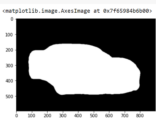
3.1: Visualizing the separated masked image
plt.imshow(person_not_person_mapping)
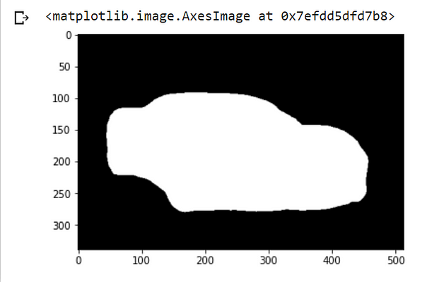
Output
As we can clearly see that the background is replaced with black color and the masked car is turned to white color as explained in the previous step, also we didn’t lose any significant information by replacing the values.
3.2: Resizing the masked image equal to the original image.
After the process of segmentation the size of the image is reduced and in our case, it’s reduced to the dimension of (300 x 500) so we will resize the image to its original dimension i.e. (900 x 596).
orig_imginal = Image.open(IMAGE_NAME)
orig_imginal = np.array(orig_imginal)mapping_resized = cv2.resize(person_not_person_mapping,
                             (orig_imginal.shape[1],
                              orig_imginal.shape[0]),
                              Image.ANTIALIAS)
mapping_resized.shape
Output
3.3: Binarization.
Due to the resizing, the image generated values ranging from 0,1,2…255, to limit the values again in between 0–255 we have to binarize the image using the Otsu’s Binarization technique. In brief, Otsu’s Binarization is an adaptive way of finding the threshold values of a grayscaled image. It goes through all possible threshold values from the range of 0-255 and finds the best possible threshold for the given image.
Internally it’s based on some statistical concepts like variance, to find out the classes based on the selected threshold. Once an optimal threshold is selected then pixel value greater than the threshold will be considered as white pixel and values lesser than the threshold is considered as a black pixel. To know more about check this article out.
gray = cv2.cvtColor(mapping_resized, cv2.COLOR_BGR2GRAY)
blurred = cv2.GaussianBlur(gray,(15,15),0)
ret3,thresholded_img = cv2.threshold(blurred,0,255,cv2.THRESH_BINARY+cv2.THRESH_OTSU)
plt.imshow(thresholded_img)
Output
The output will remain the same. There won’t be any difference compared to the previous one.
Step 4: Adding colors to the threshold image.
Now we are done with binarization it’s time to convert the grayscaled image to an RGB image.
mapping = cv2.cvtColor(thresholded_img, cv2.COLOR_GRAY2RGB)
np.unique(mapping)
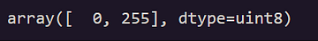
Output
In the output, after applying the colors to the image it contains two unique pixel values i.e. 0,255 using this map we will apply background blur in upcoming steps.
4.1: Applying blur to the original image.
Moving up next, let’s apply the background blur effect to our original input image.
blurred_original_image = cv2.GaussianBlur(orig_imginal,
                                          (251,251),0)
plt.imshow(blurred_original_image)

Output
4.2: Obtaining the background blur.
This is the step where when we actually blur to the background of the input image with a simple line of the code snippet.
layered_image = np.where(mapping != (0,0,0),
                         orig_imginal,
                         blurred_original_image)
plt.imshow(layered_image)
In the above snippet what we are doing is simply filling out blurred images where the pixel intensity values are 0 i.e. filling all black pixels and filling the original image where the pixel intensity values are 255 which is white pixels, Based on segmentation map. This results in a nice-looking bokeh effect show below.
Output
4.3: Finally saving the image.
Now the only thing left to do is to save the bokeh image, and we are done!
im_rgb = cv2.cvtColor(layered_image, cv2.COLOR_BGR2RGB)
cv2.imwrite("Potrait_Image.jpg", im_rgb)
5. Credits:
This article was written with reference to Bhavesh Bhatt’s video regarding the same on YouTube so hats off to him, also all the above code snippets given is only the important ones, the complete code with line by line comments is available on my GitHub page.
6. Conclusion:
To summarize, getting background blur is just one of the things that Deep Learning can do. As we make progress the models are getting better and better from classification to generating deep fakes as all of us are looking forwards to it!
About the Author