How to Use Stacking to Choose the Best Possible Algorithm?
This article was published as a part of the Data Science Blogathon.
Best features + Best algorithm = Accurate Predictions

Photo by Sam Balye on Unsplash
Every time you stumble upon a huge volume of data with thousands of features, you will be wondering what would be the best algorithm to get accurate predictions on this data, and whether to use all the features or reduce the feature space. Through this blog, I will take you through the steps in finding the good features through lasso regression and getting the right algorithm through a technique called stacking.
Selection of the best algorithm
Stacking refers to a method of joining the machine learning models, similar to arranging a stack of plates at a restaurant. It combines the output of many models. The performance of stacking is usually close to the best model and sometimes it can outperform the prediction performance of each individual model.
The objective is to get accurate predictions of the target variable, with the most relevant explanatory variables. We will do that by applying machine learning models such as Random Forest, Lasso regression, and Gradient Boosting.Then let us stack the output of these individual models and pass it to a ridge regressor to compute the final predictions. Stacking utilizes the strength of each individual model by using their output as input to the final model.
We compare the performance of the stacking regressor with individual models’ performance. The performance of stacking is usually close to the best model and sometimes it can outperform the prediction performance of each individual model. The plots at the end of this article show the performance of the individual regressors and the stacked regressor on a given data set.
Selection of the best features
The selection of variables brings many advantages. The model gets simpler, less code for error handling, and reduces the chances of the fitting, and minimizes the introduction of bugs. The execution time of the models and memory consumption is reduced.
In machine learning terminology, Least absolute shrinkage and selection operator (Lasso) is a regression analysis method that accomplishes both variable selection and regularization in order to enhance the prediction accuracy and interpretability of the model. It alters the model fitting process and selects only a subset of the covariates. It achieves this by forcing certain coefficients to be set to zero, and remove these coefficients in building the model.
Implementation
For the implementation, we will use the house price dataset available on this kaggle page. Scroll down to the bottom of the page, and click on the link ‘train.csv’, and then click the ‘download’ blue button towards the right of the screen, to download the dataset. Here the file is renamed as ‘houseprice.csv’ We build a machine learning model to predict the sale price of houses based on different explanatory variables describing various aspects of these houses. We aim to minimize the difference between the real price and the price estimated by our model.
So we are going to use the most interesting features
chosen by the Lasso regression model and check
the performance of each model individually and the stack perormance. Follow along.
Step 1: Import all the libraries
# let us import all the libraries
# to handle datasets
import numpy as np
# for plotting
import matplotlib.pyplot as plt
# to divide train and test set
from sklearn.model_selection import train_test_split
# feature scaling
from sklearn.preprocessing import MinMaxScaler
#to buid models
from sklearn.linear_model import Lasso
from sklearn.feature_selection import SelectFromModel
# models for Stacking
from sklearn.ensemble import GradientBoostingRegressor
from sklearn.ensemble import RandomForestRegressor
from sklearn.ensemble import StackingRegressor
from sklearn.linear_model import LassoCV
from sklearn.linear_model import RidgeCV
# to evaluate the model
from sklearn.metrics import mean_squared_log_error
from sklearn.metrics import mean_squared_error,r2_score
import math
#to find training time of the model
import time
# to visualise al the columns in the dataframe
pd.pandas.set_option('display.max_columns', None)
import warnings
warnings.simplefilter(action='ignore')
Step 2: Load dataset
The house price dataset contains 1460 rows, i.e., houses, and 81 columns, i.e., variables.
Python Code:
Step 3: Data Engineering
Data needs to be engineered to handle:
- Treat missing values
- Categorical variables: Remove rare labels
- Categorical variables encoding
- Engineer temporal variables
- Treat non-Gaussian distributed variables
- Feature scaling
Before beginning to engineer our features, we separate the data into training and testing set. Because when we engineer features, some techniques learn parameters from data. It is important to learn these parameters only from the train set to avoid over-fitting. Further, we need to set the seed wherever we expect randomness.
# Let's separate into train and test set
# Remember to set the seed (random_state for this sklearn function)
X_train, X_test, y_train, y_test = train_test_split(data,data['SalePrice'],test_size=0.25,
                                                     random_state=0)
X_train.shape, X_test.shape
Treat Missing values
We will find the missing values in numerical variables, and replace them with the mode.
 replace missing values with mode
# make a list with the numerical variables that contain missing values
vars_with_na = [var for var in data.columns if X_train[var].isnull().sum() > 0 and X_train[var].dtypes != 'O']
for var in vars_with_na:
    # calculate the mode using the train set
    mode_val = X_train[var].mode()[0]
    # replace missing values by the mode
    # (in train and test)
    X_train[var] = X_train[var].fillna(mode_val)
    X_test[var] = X_test[var].fillna(mode_val)
Make a list of the categorical variables that contain missing values and replace them with the label ‘Missing’
# make a list of the categorical variables that contain missing values vars_with_na = [var for var in data.columns if X_train[var].isnull().sum() > 0 and X_train[var].dtypes == 'O'] # replace missing values with new label: "Missing" X_train[vars_with_na] = X_train[vars_with_na].fillna('Missing') X_test[vars_with_na] = X_test[vars_with_na].fillna('Missing')-
Categorical-Removing rare labels
First, we will isolate those categories within variables that are present in less than 1% of the observations. That is, all values of categorical variables that are shared by less than 1% of houses will be named as “Rare”.
# let's capture the categorical variables in a list cat_vars = [var for var in X_train.columns if X_train[var].dtype == 'O'] def find_frequent_labels(df, var, rare_perc): # find_frequent_labels function finds the labels that are shared by more than # a certain % of the houses in the dataset df = df.copy() tmp = df.groupby(var)['SalePrice'].count() / len(df) return tmp[tmp > rare_perc].index for var in cat_vars: # find the frequent categories frequent_ls = find_frequent_labels(X_train, var, 0.01) # replace rare categories by the string "Rare" X_train[var] = np.where(X_train[var].isin(frequent_ls), X_train[var], 'Rare') X_test[var] = np.where(X_test[var].isin(frequent_ls), X_test[var], 'Rare') -
Categorical variable encoding
Next, we will write a small function that assigns discrete values to the strings of the variables. For instance, the smaller value corresponds to the category that shows a smaller mean house sale price.
def replace_categories(train, test, var, target): # order the categories in a variable from that with the lowest # house sale price, to that with the highest ordered_labels = train.groupby([var])[target].mean().sort_values().index # create a dictionary of ordered categories to integer values ordinal_label = {k: i for i, k in enumerate(ordered_labels, 0)} # use the dictionary to replace the categorical strings by integers train[var] = train[var].map(ordinal_label) test[var] = test[var].map(ordinal_label) for var in cat_vars: replace_categories(X_train, X_test, var, 'SalePrice') -
Engineer temporal variables
There are 4 variables that refer to the years in which the house or the garage was built or remodeled. We will capture the time elapsed between those variables and the year in which the house was sold:
def elapsed_years(df, var): # capture difference between the year variable # and the year in which the house was sold df[var] = df['YrSold'] - df[var] return df for var in ['YearBuilt', 'YearRemodAdd', 'GarageYrBlt']: X_train = elapsed_years(X_train, var) X_test = elapsed_years(X_test, var) -
Treat non-gaussian distributed variables
Some variables show skewed distribution. We will log transform the positive numerical variables in order to get a more Gaussian-like distribution. This will help linear machine learning models.
for var in ['LotFrontage', 'LotArea', '1stFlrSF', 'GrLivArea', 'SalePrice']: X_train[var] = np.log(X_train[var]) X_test[var] = np.log(X_test[var]) -
Feature Scaling
For use in linear models, features need to be either scaled or normalized. We will scale features to the minimum and maximum values.
# capture all variables in a list
# except the target and the ID
train_vars = [var for var in X_train.columns if var not in ['Id', 'SalePrice']]
# create scaler
scaler = MinMaxScaler()
#  fit  the scaler to the train set
scaler.fit(X_train[train_vars])
# transform the train and test set
X_train[train_vars] = scaler.transform(X_train[train_vars])
X_test[train_vars] = scaler.transform(X_test[train_vars])
print(X_train.isnull().sum().any(),X_test.isnull().sum().any())
We finished the formal feature engineering steps. You can extend these feature engineering steps. For example removal of outliers etc.
Step 4: Feature Selection
We will select variables using the Lasso regression: Lasso has the property of setting the coefficient of non-informative variables to zero. This way we can identify those variables and remove them from our final model. In the following cells, we will select a group of variables, the most predictive ones, to build our machine learning model.
# capture the target (notice that the target is log transformed)
y_train = X_train['SalePrice']
y_test = X_test['SalePrice']
# drop unnecessary variables from our training and testing sets
X_train.drop(['Id', 'SalePrice'], axis=1, inplace=True)
X_test.drop(['Id', 'SalePrice'], axis=1, inplace=True)
Let’s go ahead and select a subset of the most predictive features. There is an element of randomness in the Lasso regression, so remember to set the seed.Select a suitable alpha (the equivalent of penalty).The bigger the alpha the less number of features will be selected.
sel_= SelectFromModel(Lasso(alpha=0.005,random_state=0))
# train Lasso model and select features
sel_.fit(X_train,y_train)
# let's print the number of total and selected features
selected_feats = X_train.columns[(sel_.get_support())]
# let's print some stats
print('Total features: {}'.format((X_train.shape[1])))
print('selected features: {}'.format(len(selected_feats)))
print('features with coefficients shrank to zero: {}'.format(np.sum(sel_.estimator_.coef_== 0)))
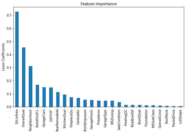
25 out of 79 features are selected.Let us have a look at the important features.
#let's look at the feature importance
importance = pd.Series(np.abs(lin_model.coef_.ravel()))
importance.index = selected_feats
importance.sort_values(inplace=True, ascending=False)
importance.plot.bar(figsize=(10,6))
plt.ylabel('Lasso Coefficients')
plt.title('Feature Importance')
Step 5: Build models
Extract the selected features.
X_train=X_train[selected_feats]
X_test=X_test[selected_feats]
print(X_train.shape,X_test.shape)
We will define our models. There is no limit for
adding the models in the stack.
# The parameters inside the models can be varied
params = {'n_estimators': 500,
          'max_depth': 4,
          'min_samples_split': 5,
          'learning_rate': 0.01,
          'loss': 'ls'}
GB_model= GradientBoostingRegressor(**params)
lin_model = Lasso(alpha=0.005, random_state=0)
RF_model = RandomForestRegressor(n_estimators=400,random_state=0)
# Get these models in a list
estimators = [('Random Forest', RF_model),
              ('Lasso', lin_model),
              ('Gradient Boosting', GB_model)]
#Stack these models with StackingRegressor
stacking_regressor = StackingRegressor(estimators=estimators,
                                       final_estimator=RidgeCV())
Step 6: Compare the performance
We will compare the performance with the help of scatter plots
def plot_regression_results(ax, y_true, y_pred, title, scores, elapsed_time):
    """Scatter plot of the predicted vs true targets."""
    ax.plot([y_true.min(), y_true.max()],
            [y_true.min(), y_true.max()],
            '--r', linewidth=2)
    ax.scatter(y_true, y_pred, alpha=0.2)

    ax.spines['top'].set_visible(False)
    ax.spines['right'].set_visible(False)
    ax.get_xaxis().tick_bottom()
    ax.get_yaxis().tick_left()
    ax.spines['left'].set_position(('outward', 10))
    ax.spines['bottom'].set_position(('outward', 10))
    ax.set_xlim([y_true.min(), y_true.max()])
    ax.set_ylim([y_true.min(), y_true.max()])
    ax.set_xlabel('True_Price')
    ax.set_ylabel('Predicted_Price')
    extra = plt.Rectangle((0, 0), 0, 0, fc="w", fill=False,
                          edgecolor='none', linewidth=0)
    ax.legend([extra], [scores], loc='upper left')
    title = title + 'n Evaluation in {:.2f} seconds'.format(elapsed_time)
    ax.set_title(title)
fig, axs = plt.subplots(2, 2,figsize=(9, 7)) axs = np.ravel(axs) errors_list=[] for ax, (name, est) in zip(axs , estimators + [('Stacking Regressor', stacking_regressor)]): start_time = time.time() model = est.fit(X_train, y_ train) elapsed_time = time.time() - s tart_time pred = model.predict(X_test) errors = y_test - model.predic t(X_test) errors_list.append(errors) test_r2= r2_score(np.exp(y_ test), np.exp(pred)) test_rmsle=math.sqrt(mean_ squared_log_error(y_test,pred) ) plot_regression_results(ax,y_ test,pred,name,(r'$R^2={:.3f}$ ' + '\n' + r'$RMSLE={:.3f}$').format(test _r2,test_rmsle),elapsed_time) plt.tight_layout() plt.subplots_adjust(top=0.9) plt.show()
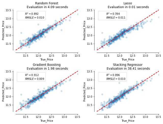
By looking at the plots, we observe that the gradient boosting model performs well, and the stacking regressor is closer to the gradient boosting model in performance.
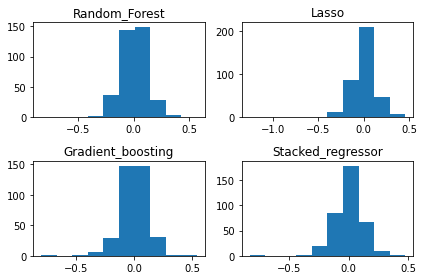
Let us see the distribution of errors of each of these models.
titles = ['Random_Forest','Lasso','Gradient_boosting','Stacked_regressor']
f,a = plt.subplots(2,2)
a = a.ravel()
for idx,ax in enumerate(a):
    ax.hist(errors_list[idx])
    ax.set_title(titles[idx])
plt.tight_layout()
#let's look at the feature importance importance = pd.Series(np.abs(lin_model.coef_.ravel())) importance.index = selected_ feats importance.sort_values(inplace =True, ascending=False) importance.plot.bar(figsize=(1 0,6)) plt.ylabel('Lasso Coefficients') plt.title('Feature Importance')
The distribution of the errors follows quite closely a gaussian distribution. That suggests that our models are doing a good job in making predictions.
Thanks for reading. Like, share, and write your thoughts.
References:
1. Tibshirani, Robert(1996) “Regression Shrinkage and Selection via the lasso” Journal of the Royal Statistical Society. Series B (Methodological) Vol. 58, No. 1 (1996), pp. 267-288 (22 pages)Published By Wiley https://www.jstor.org/stable/2346178
2. https://scikit-learn.org/stable/auto_examples/ensemble/plot_stack_predictors.html


Hello: I received your email on this blog post and decided to check it out. I copied the code into Spyder but got an error when the program attempted to plot the results. The error is on the following line: ax.hist(errors_list[idx]) Thanks, Manny
In the step 6, defining "plot_regression_results" function code shows twice. Also the last code "Let us see the distribution of errors of each of these models." parts, variable "error_list" is not defined. I think second "plot_regression_results" code have to be fixed for defining "error_list " variable and the using example of "plot_regression_result" function have to be added
In the step 6, defining "plot_regression_results" function code shows twice. Also the last code "Let us see the distribution of errors of each of these models." parts, variable "error_list" is not defined. I think second "plot_regression_results" code have to be fixed for defining "error_list " variable and the using example of "plot_regression_result" function have to be added.
Code has been modified. Execute the feature importance section at the end.