Deployment of ML models in Cloud – AWS SageMaker (in-built algorithms)
Introduction:
Gone are the days when enterprises set up their own in-house server and spending a gigantic amount of budget on storage infrastructure & maintenance. With the introduction of Cloud computing technologies from key players(Amazon, Google & Microsoft) and many other budding competitors, companies are migrating towards the serverless platform. This bright idea assists the organizations to focus on their core business strategies.
The main theme of this article is the machine learning service(Sagemaker) provided by Amazon(AWS) and how to leverage the in-built algorithms available in Sagemaker to train, test, and deploy the models in AWS.
AWS SageMaker is a fully managed Machine Learning service provided by Amazon. The target users of the service are ML developers and data scientists, who want to build machine learning models and deploy them in the cloud. However, one need not be concerned about the underlying infrastructure during the model deployment as it will be seamlessly handled by the AWS.
Any concept can be conveyed in a clear-cut manner when applied to a real-life problem. So, let’s pull the loan prediction challenge posted in Analytics Vidhya. Based on different input predictors, the goal is to forecast whether the Loan should be approved or not for a customer.
Table of Contents
1. Creating a Notebook Instance
2. Loading Datasets, EDA & Train validation split
3. Dataset upload in s3 bucket
4. Training Process
5. Model Deployment and Endpoint creation
Step1- Creating a Notebook Instance: The whole process kicks start by creating a notebook instance where a virtual machine(EC2 — Elastic cloud) and storage(EBS volume) get allocated for our objective. It is the user’s choice to pick the type & size of the EC2 as well as the capacity of EBS volume. In order to perform huge computations, additional virtual instances can be appended on top of the regular EC2. Once the task is completed, the EC2 instance can be turned off by clicking on the ‘STOP’ under actions. On the other hand, the EBS volume still holds the data assigned even though the virtual machine is not in use.
For learning purposes, an account can be created under a free trial, and ‘Amazon SageMaker’ should be pulled from the services. The region can be chosen from the top right corner. Under the ‘Notebook instances’ in the AWS SageMaker, click on the ‘create notebook instance’.
Note: The reasons for having different regions are to comply with the GDPR rules and also closer the region to client location better the speed.
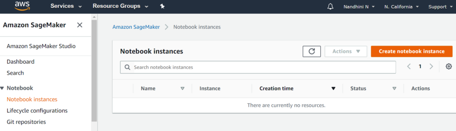 Fig1 — shows ‘Create notebook instance’ & region as ‘N.California’
The “create notebook instance” is followed by allocating the EC2 instances and EBS volume.
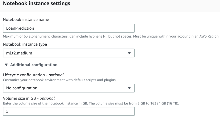
Fig2 — shows EC2 instance & EBS volume
The final process in this step is to assign an access role, as notebook instances require permission to call other services including SageMaker and S3(another memory storage discussed below).

Fig3 — shows the role of access
Step2 — Loading Datasets, EDA & Train validation split: Now that we have allocated a virtual machine for our goal and the subsequent step would be to create folders, datasets, and notebooks. Here we upload the datasets (train & test), perform exploratory data analysis for the training dataset, and split the training dataset into training and validation sets. As we want to tune the hyperparameters based on the performance of the validation set.
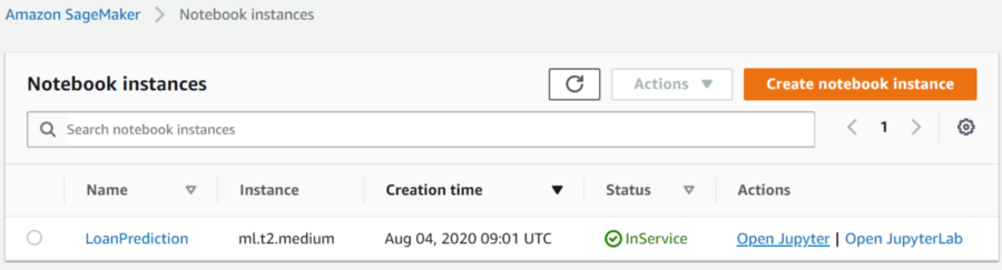
Fig4 — shows the notebook instance created
By clicking on ‘Open Jupyter’ a new window opens where we can create a folder for our project.
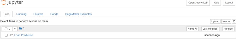
Fig5 — shows the folder “Loan Prediction”
We can double click on the folder and load the train, test datasets, and also the exploratory data analysis that has been already done in the local machine. AWS Sagemaker does not require the headers during the training process and also the target column should be the first column in the data frame.
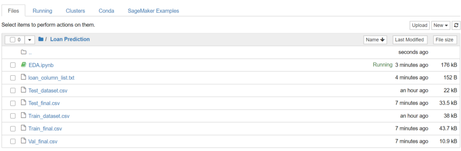
Fig6 — shows the list of files split after the EDA process
Step3 — Dataset upload in S3 bucket: Before we start the training, all the datasets (train, validation, and test) should be uploaded into the S3 bucket from where the details are retrieved during the training. S3 buckets are basically simple storage cloud services offered by Amazon. Amazon S3 buckets, which are similar to file folders, store objects, which consist of data and its descriptive metadata(taken from the original description). We can create an S3 bucket for our process by clicking on the ‘S3’ under AWS services and giving name, region respectively. The S3 bucket should also be in the same region as the notebook instance.
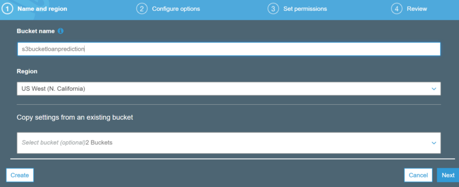
Fig7 — shows the S3 bucket name and the region
The below python code shows how to place all the datasets in the ‘S3’ bucket. There might be some unfamiliar terms such as ‘boto3’, these are libraries designed for AWS services.
#boto3 => Pyhton library for calling up AWS services
import boto3
import sagemaker
from sagemaker import get_execution_role
#provide the name and location of the files to be stored in the S3 bucket
bucket_name = 's3bucketloanprediction'
train_file_name = 'Loan Prediction/Train_final.csv'
val_file_name = 'Loan Prediction/Val_final.csv'
test_file_name = 'Loan Prediction/Test_final.csv'

model_output_location = r's3://{0}/LoanPrediction/model'.format(bucket_name)
train_file_location = r's3://{0}/{1}'.format(bucket_name, train_file_name)
val_file_location = r's3://{0}/{1}'.format(bucket_name, val_file_name)
test_file_location = r's3://{0}/{1}'.format(bucket_name, test_file_name)
#define a method for writing into s3 bucket
def write_to_s3(filename, bucket, key):
    with open(filename, 'rb') as f:
        return boto3.Session().resource('s3').Bucket(bucket).Object(key).upload_fileobj(f)
write_to_s3('Train_final.csv', bucket_name, train_file_name)
write_to_s3('Val_final.csv', bucket_name, val_file_name)
write_to_s3('Test_final.csv', bucket_name, test_file_name)
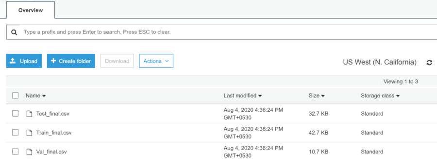
Fig8 — shows the files moved to the s3 bucket
All the datasets are successfully uploaded into the given s3 bucket.
Step4 — Training Process: Since we are using in-built algorithms, we need to make a call to those algorithms for training. These algorithms are stored as containers in ECR (Elastic Container Registry) which are maintained for each region. By giving the path of these containers in the code, these algorithms will be called. The region-wise registry path details can be found in the link.
For instance, if we want to use XGBoost Classifier from the region US West (N. California), the docker container path is ‘746614075791.dkr.ecr.us-west-1.amazonaws.com’. The subsequent step is building the model using the docker container from ECR.
Once the training process is complete, the updated model with finalized weights and bias is stored in the s3 bucket as per the instructions provided.
#provide the ECR container path since we are using north california
container = {'us-west-1': '746614075791.dkr.ecr.us-west-1.amazonaws.com/sagemaker-xgboost:1.0-1-cpu-py3'}
#create a sagemaker session
sess = sagemaker.Session()
bucket_name = 's3bucketloanprediction'
model_output_location = r's3://{0}/LoanPrediction/model'.format(bucket_name)
estimator = sagemaker.estimator.Estimator(container[boto3.Session().region_name],
                                          role,
                                          train_instance_count = 1,
                                          train_instance_type='ml.m4.xlarge',
                                          output_path = model_output_location,
                                          sagemaker_session = sess,
                                          base_job_name = 'xgboost-loanprediction'
                                         )
The container has the details of the algorithm path, role basically allows the notebook to access s3 and Sagemaker. Here, the training machine(train_instance_type) should be explicitly specified based on the computational requirement. The count defines the number of machines we need during the training. If it demands huge computations, then larger machines must be allocated. Finally, the path specified in the output_path holds the finalized model. During the training, the algorithm is accessed from ECR and the datasets are retrieved from the s3 bucket.
Hyperparameters corresponding to each algorithm has to be set before we fit the model. There are white papers that contain the list of hyperparameters and the corresponding details.
#setting hyperparameters corresponding to the XGBoost algorithm
estimator.set_hyperparameters(max_depth=5,
                              objective = 'binary:logistic',
                              eta=0.1,
                              subsample=0.7,
                              num_round=10,
                              eval_metric = 'auc')
#training the model using fit model
training_file = sagemaker.session.s3_input(s3_data=train_file_location, content_type = "csv")
validation_file = sagemaker.session.s3_input(s3_data=val_file_location, content_type = "csv")
data_channels = {'train':training_file, 'validation':validation_file}
estimator.fit(inputs=data_channels, logs=True)
Once the fit command is issued with train and validation files, a separate GPU allocated in the training instance will be pulled up and the training will kick start. The training jobs can be monitored under ‘Training’ -> ‘Training jobs’. After the completion of the training, the performance results are displayed based on the evaluation metrics mentioned in the hyperparameter section.
Step5 — Model Deployment and Endpoint Creation: The final step in the whole process is deploying the finalized model and creating an endpoint that will be accessed by external interfaces. The machine allocated in the endpoint will be in a running state and the cost will be deduced accordingly. So, when other external applications are not using it, then the endpoint should be removed using the delete option.
#deploying the model and create an end point
predictor = estimator.deploy(initial_instance_count = 1,
                             instance_type = 'ml.m4.xlarge',
                             endpoint_name = 'xgboost-loanprediction-ver1')
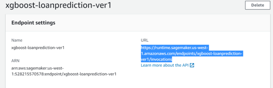
Fig9 — shows the URL accessed from an external application
Using the delete option at the top right corner, the endpoint could be removed.
The entire code and the datasets can be found in the Github repository link.
Conclusion:
So far we have discussed one of the options of building an ML model in AWS Sagemaker using built-in algorithms. The next step would be to use our own model rather than the one already present in the ECR that comes with Sagemaker. Below are my recommendations to get valuable insights on how to deploy custom models into AWS.


