Text Mining Simplified – IPL 2020 Tweet Analysis with R

This article was published as a part of the Data Science Blogathon.

Introduction

Text mining utilizes different AI technologies to automatically process data and generate valuable insights, enabling companies to make data-driven decisions.

Text mining identifies facts, relationships, and assertions that would otherwise remain buried in the mass of textual big data. Once extracted, this information is converted into a structured form that can be further analyzed, or presented directly using clustered HTML tables, mind maps, charts, etc.

Text Mining tools and techniques are rapidly penetrating industries right from academia and healthcare to businesses and social media platforms. Here are a few most common text mining applications around us:

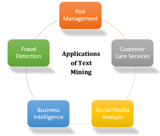
Risk Management: One of the primary causes of failure in the business sector is the lack of proper risk analysis. Since text mining tools and technologies can gather relevant information from thousands of text data sources and create links between the extracted insights, it allows companies to access the right information at the right moment and boost their abilities to mitigate potential risks.

Fraud Detection: Finance and Insurance companies mainly utilizes this opportunity. By combining the outcomes of text analyses with relevant structured data these companies process claims swiftly as well as detects and prevents fraud more efficiently.

Business Intelligence: Apart from providing profound insights into customer behavior and trends, text mining techniques also help companies to analyze the strengths and weaknesses of their rivals, thus, giving them a competitive advantage in the market.

Social Media Analysis: There are many text mining tools designed exclusively for analyzing the performance of social media platforms. These help to track and interpret the texts from news, blogs, emails, etc. Also, text mining tools can efficiently analyze the number of posts, likes, and followers on social media, thereby allowing people to understand the reaction of netizens who are interacting with their brand and online content. This analysis enables social media platforms to understand ‘what’s hot and what’s not’ for their target audience.

Customer Care Services: Text mining techniques like Natural Language Processing (NLP), are getting increasing importance in the field of customer care. Companies are investing in text analytics software to enhance their overall customer experience by accessing the textual data from surveys, customer feedback,  calls, etc. aiming to a sharp reduction in the response time of the company.

Now, let us consider a case study for a better illustration of how actually text mining works and how to create word clouds using text mining, reasons one should use word clouds to present text data.

Case Study – IPL 2020 Tweet Analysis

This case study can be seen as an example of Social Media Analysis as mentioned above. Here, I  will process with Tweets about Indian Premier League IPL 2020 by following the link here.

“Text Mining is a technique that boosts the research process and helps to test the queries.”

For analysis, I will be using R and R studio, a language and environment for statistical computing and graphics. Why R?  R provides a wide variety of statistical and graphical techniques and has a rich set of packages for Natural Language Processing (NLP) and generating plots, as well as for foundational steps involving loading the text file into a corpus, then cleaning and stemming the data before performing analysis. Moreover, It is open-source and easy to learn.

So, without any further discussion let’s dive deep into our case study.

 Import and Quick look of Dataset

Our dataset IPL_Tweets  consists of 20231 observations and 19 variables. I used the read.csv() command for importing dataset; read.csv() is used for reading comma-separated value (csv) files, where a comma “,” is used as a field separator.

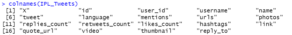
The variable names are obtained as:

colnames(IPL_Tweets)

Next, we will check for null values and duplicate values in the dataset.

anyNA(IPL_Tweets)  #checking for missing values

sum(duplicated(IPL_Tweets))   #search for duplicate values

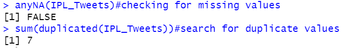
Removing duplicate entries is a key step for effective data analysis. Our dataset has 7 duplicate values which is removed using code as-

IPL_Tweets=IPL_Tweets[duplicated(IPL_Tweets)!= "TRUE",]  #Duplicated entries are removed

Although we have 19 variables in our dataset but to keep things simple we will retrieve only tweets and corresponding hashtags into two separate files named Tweets and Hashtags respectively using-

rownumbers=c(1:nrow(IPL_Tweets))

Tweets=data.frame(doc_id=rownumbers,text=IPL_Tweets$tweet)

Hashtags= data.frame(doc_id=rownumbers, text=IPL_Tweets$hashtags)

Let’s have a look at our Tweets and Hashtags.

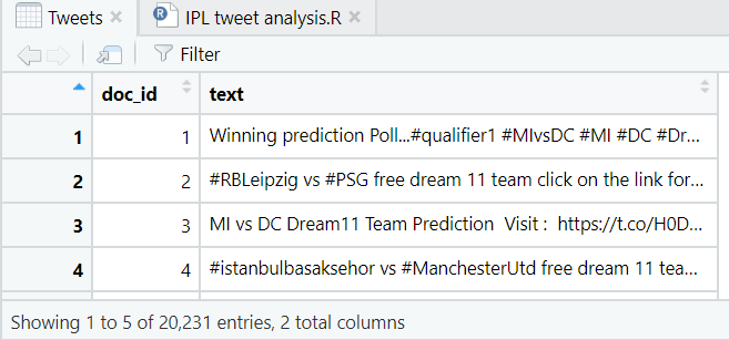
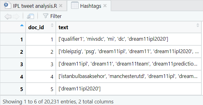
Tweets without any hashtags are common. So, it is evident that the Hashtags dataset have some missing entries, hence, we will remove those as well using-

Hashtags=Hashtags[Hashtags$text!= "[]",]

After performing all the steps here, we have Tweets with 20231 observations and 2 columns and Hashtags with 19971 observations and 2 columns.

Installing and Loading R Packages

The following packages are used in the case study in this article:

• tm for text mining operations like removing numbers, special characters, punctuations and stop words.
• snowballc for stemming, which is the process of reducing words to their base or root form, for example, a stemming algorithm would reduce the words “fishing”, “fished” and “fisher” to the stem “fish”.
• wordcloud and wordcloud2 for generating the word cloud plot.
• RColorBrewer for color palettes used in various plots.

# Install
install.packages("tm")  # for text mining
install.packages("SnowballC") # for text stemming
install.packages("wordcloud") # word-cloud generator
install.packages("RColorBrewer") # color palettes
install.packages("wordcloud2") # Word-cloud generator

 # Load
library("tm")
library("SnowballC")
library("wordcloud")
library("RColorBrewer")
library(wordcloud2)

Cleaning Up Text Data

The next thing we do is to construct a Corpus out of the datasets and process it. In R, a Corpus is a collection of a text document(s) to apply text mining or NLP routines on.

TextCorpus= Corpus(DataframeSource(Tweets)) #Corpus for Tweets  
Hashcorpus=Corpus(DataframeSource(Hashtags)) #Corpus for Hashtags

Since the dataset is obtained in a raw format, thus we will have a lot of unwanted stuff in the dataset which can hamper our objective of analyzing the data. In the following steps, we will be cleaning and processing the data in order to conduct the analysis in the later section.

1. Converting all words into lowercase.
2. Removing punctuations and numbers.
3. Removing stop words.
4. Eliminating extra white space.
5. Lastly, text stemming.

First, we will convert all the words and sentences in the corpus into lower case. One can also use uppercase but conventionally lower case is used. This step reduces the chances of treating the same words as different unique words, e.g. “Mining” and “mining” are treated as different words even though they are the same, so here keeping them in lowercase resolves that.

#Converting to lowercase
TextCorpus1=tm_map(TextCorpus,content_transformer(tolower)) # for Tweets
Hashcorpus1=tm_map(Hashcorpus,content_transformer(tolower)) #for Hashtags

Next, to remove the punctuations from the corpus we execute the following code, otherwise, these will be considered as individual text elements during the analysis, which will come in the result without any sentiments attached to it. Similarly, there is no requirement to keep numbers if any in the dataset, hence the given below code can be executed to remove numbers from the data.

#removing punctuation
TextCorpus2=tm_map(TextCorpus1,content_transformer(removePunctuation))
Hashcorpus2=tm_map(Hashcorpus1,content_transformer(removePunctuation))
#removing number
TextCorpus3=tm_map(TextCorpus2,content_transformer(removeNumbers))
Hashcorpus3=tm_map(Hashcorpus2,content_transformer(removeNumbers))

The next thing we have to address is the presence of stop words. Often there are words that are frequent but provide little information. These are called stop words, and you may want to remove them from your analysis. Some common English stop words include “I”, “she’ll”, “the”, etc. In the tm package, there are 174 common English stop words.

#removing stopwords
TextCorpus4=tm_map(TextCorpus3,content_transformer(removeWords),stopwords())
Hashcorpus4=tm_map(Hashcorpus3,content_transformer(removeWords), stopwords())

The next step is to eliminate extra white space between words in the corpus.

#Removing Spaces between words
TextCorpus5 = tm_map (TextCorpus4, stripWhitespace)
HashCorpus5= tm_map(HashCorpus4,stripWhitespace)

Last but not least, text stemming. It is the process of reducing the word to its root form. The stemming process simplifies the word to its common origin. For example, the stemming process reduces the words “fishing”, “fished” and “fisher” to its stem “fish”.

# Text stemming - which reduces words to their root form
TextCorpus6= tm_map(TextCorpus5,stemDocument)
HashCorpus6= tm_map(HashCorpus5,stemDocument)

Now, our text dataset is ready for further analysis.

 Creation of Document Term Matrix

A Document-term matrix or term-document matrix is a mathematical matrix that describes the frequency of terms that occur in a collection of documents. In a document-term matrix, rows correspond to documents in the collection and columns correspond to terms.

When creating a database of terms that appear in a set of documents the document-term matrix contains rows corresponding to the documents and columns corresponding to the terms. For instance, if one has the following two (short) documents:
• D1 = “I like databases”
• D2 = “I hate databases”

then the document-term matrix would be:

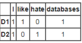
which shows which documents contain which terms and how many times they appear. In R script, the following code is used to create a document term matrix.

#Building the Term Document Matrix for Tweets
DTM= DocumentTermMatrix(TextCorpus6)
DTM=as.matrix(DTM) #Converting into a double matrix
DTM.totalfreq=colSums(DTM) # calculate the term frequencies
summary(DTM.totalfreq) #summary calculation

 

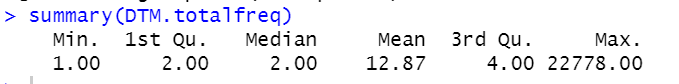
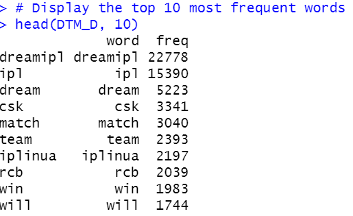
The summary statistics show the document term matrix of tweets has words with a mean frequency of 12.87 and a maximum frequency of 22778.

A similar method is followed for hashtags as well.

#Building the Term Document Matrix for Hashtags
DTM1= DocumentTermMatrix(HashCorpus6)
DTM1=as.matrix(DTM1)
DTM1.totalfreq=colSums(DTM1)
summary(DTM1.totalfreq)

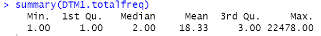
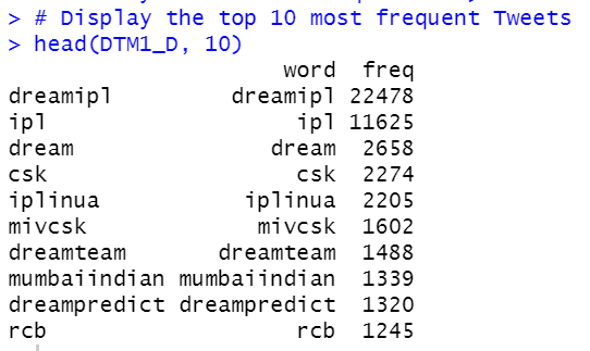
Summary stats for document term matrix of hashtags has hashtags with a mean frequency of 18.33 and a maximum frequency of 22478.

 Finding Most Frequent Words

After creating a Document-term Matrix, plotting the top 10 most frequent words using a bar chart is a good basic way to visualize this word’s frequent data.

So, ready to find out what is #Trending in IPL 2020? Let’s see !!

Here, the first words are sorted by decreasing value of frequency and then plotted.

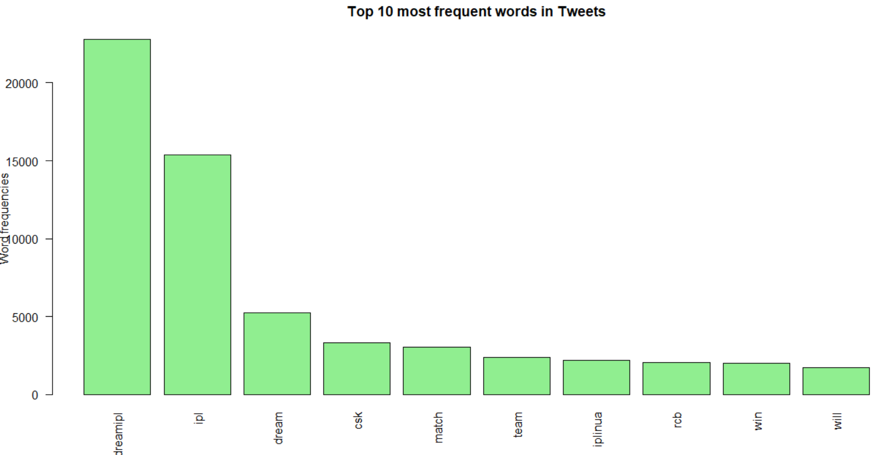
#Finding out the most frequent words in Tweets 
#Sort by descending value of frequency
DTM_V=sort(DTM.totalfreq,decreasing=TRUE)
DTM_D=data.frame(word = names(DTM_V),freq=DTM_V)
# Display the top 10 most frequent words
head(DTM_D, 10)
# Plot the most frequent words
barplot(DTM_D[1:10,]$freq, las = 2, names.arg = DTM_D[1:10,]$word,
            col ="lightgreen", main ="Top 10 most frequent words in Tweets",
                ylab = "Word frequencies")

It comes with the following outputs as-

The same process is followed to get the top 10 most frequent hashtags as well.

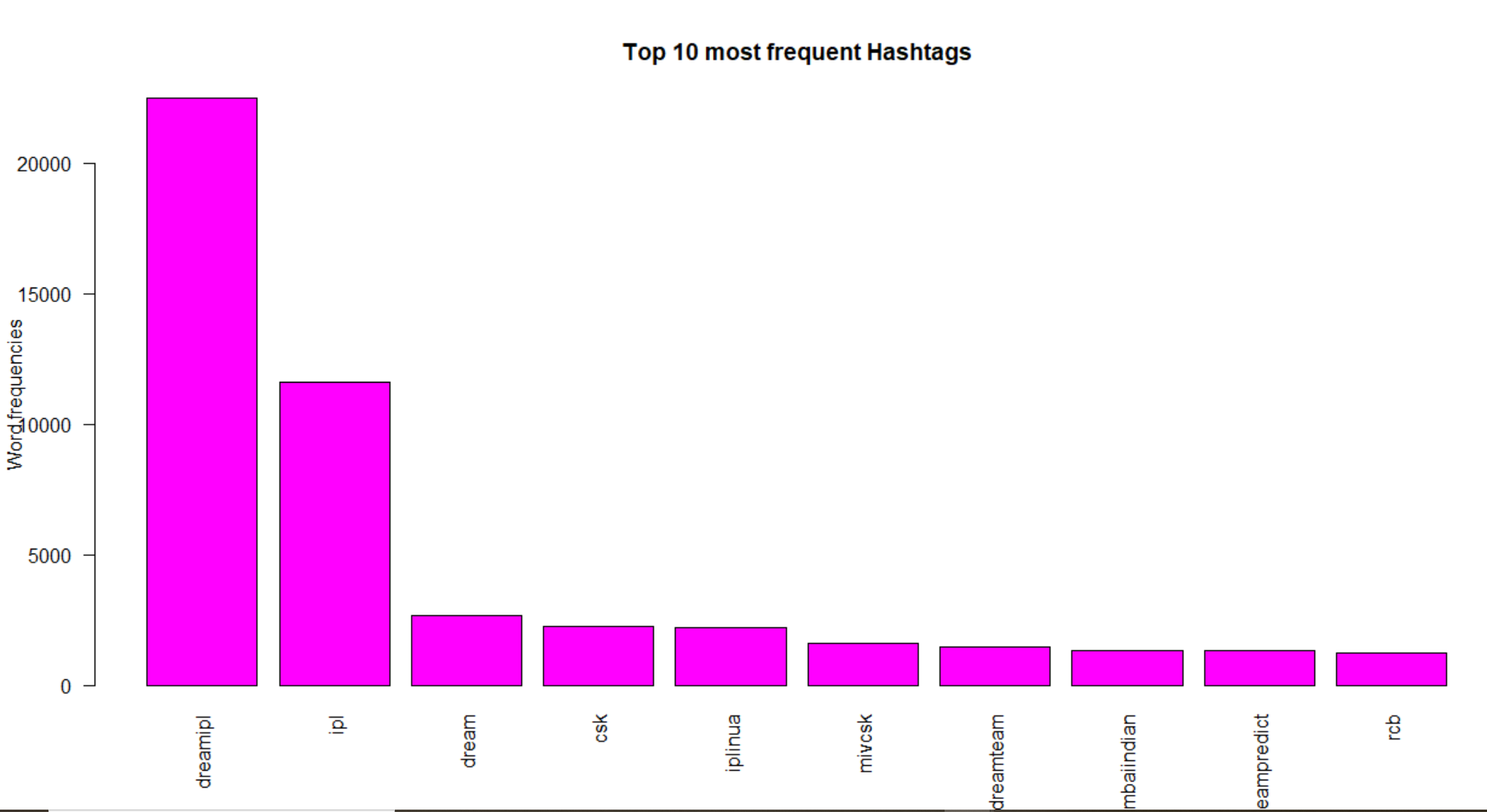
One could interpret the following from this bar chart:

• Words like, “dreamipl” is the most frequently occurring word in both tweets as well as among hashtags followed by “ipl” ,”dream” and “csk”.
•  Word “rcb” is more frequent in tweets than hashtags. The opposite goes for “iplinua”.

 Generate the Word Cloud

A word cloud is one of the most popular ways to visualize and analyze qualitative data. The feature of words can be illustrated as a word cloud as follows :

• Word clouds add clarity and simplicity.
• The most used keywords stand out better in a word cloud.
• Word clouds are a dynamic tool for communication. Easy to understand, to be shared, and are impressive words representation.

wordcloud(words = colnames(DTM),freq=DTM.totalfreq,min.freq = 500,scale =c(5,0.5),
           max.words=200,rot.per=0.30,colors=brewer.pal(n=8,"Dark2"), random.order=F)

The above code is used to create a word cloud for IPL 2020 Tweets.

In the wordcloud function we have some arguments whose implementation is briefly described below:

• Words – to fetch the collection of words to design the wordcloud
• Freq – this is to get the frequency of the terms
• Min.freq – the minimum frequency term which will be in the wordcloud
• Max.words –  maximum words in the word cloud.
• Scale – font size of the maximum to minimum frequency terms
• Colors – to add color to the words in the wordcloud
• rot.per – the percentage of words that are displayed as vertical text (with 90-degree rotation). I have set it 0.30 (30%), please feel free to adjust this setting to suit your preferences.

 

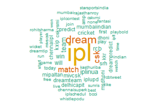
Fig 7: Word Cloud for IPL 2020 Tweets

Another wordcloud is created with help of “wordcloud2” package. Wordcloud2 offers more options to get more creative and colorful word clouds than the first one. Here, the wordcloud for IPL 2020 Tweets created from “wordcloud2”.

#word cloud 2
wordcloud2(data=DTM_D,size = 3, color = "random-light", backgroundColor = "white")

The above code creates a new word cloud as-

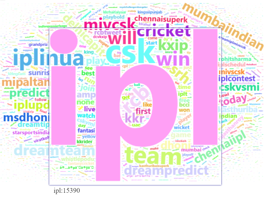
Fig 8 :Word Cloud for IPL 2020 Tweets with word cloud 2

The word cloud shows additional words that occur frequently and could be of interest for further analysis. Words like “mumbaiindian”, “mivcsk”, “kxip” etc. could provide more context around the most frequently occurring words and help to gain a better understanding of the main themes.

Lastly, we will calculate word association. This technique can be used effectively to analyze which words occur most often in association with the most frequently occurring words in the survey responses, which helps to see the context around these words. 

# Find associations 
findAssocs(DocumentTermMatrix(TextCorpus6), terms = c("ipl","dream","csk"), corlimit = 0.25)

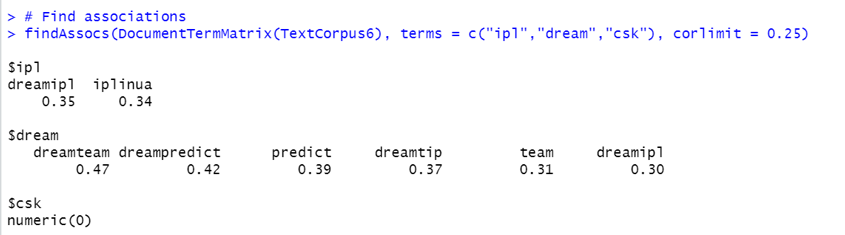
This script shows which words are associated with the most frequent words “ipl”,”dream” and “csk” with minimum correlation 25%.

Conclusion

Text mining or text analytics is a booming technology but still the results and depth of analysis vary from business to business. This article briefs about reading text data, cleaning text data, and transformations. It demonstrated how to create a word frequency table and plot a word cloud, to identify prominent themes occurring in the text. Lastly, highlighted word association analysis using correlation, helped to gain context around the prominent themes.

Link to my LinkedIn Profile:

Samprita Das 19 Nov 2020