Managed By Energy Market Authority
Frequency Annual
Source(s) Energy Market Authority
License Singapore Open Data Licence
This article was published as a part of the Data Science Blogathon.
Anomaly detection is a process in Data Science that deals with identifying data points that deviate from a dataset’s usual behavior. Anomalous data can indicate critical incidents, such as financial fraud, a software issue, or potential opportunities, like a change in end-user buying patterns.
The entire process of Anomaly Detection for a time-series takes place across 3 steps:
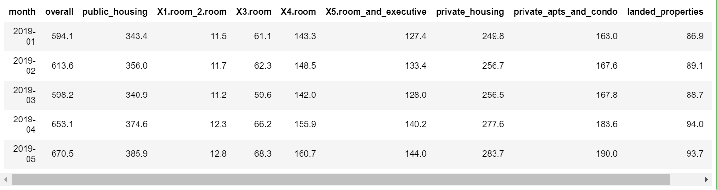
Let us download the dataset from the Singapore Government’s website that is easily accessible.- Total Household Electricity Consumption by Dwelling Type. Singapore’s government data website is quite easily downloadable. This dataset shows total household electricity consumption by dwelling type (in GWh).
In this exercise, we are going to work with 2 key packages for time series anomaly detection in R: anomalize and timetk. These require that the object be created as a time tibble, so we will load the tibble packages too. Let us first install and load these libraries.
pkg <- c('tidyverse','tibbletime','anomalize','timetk')
install.packages(pkg)
library(tidyverse)
library(tibbletime)
library(anomalize)
library(timetk)
In the previous step, we have downloaded the total electricity consumption file by dwelling type (in GWh) from the Singapore Government’s website. Let us load the CSV file into an R dataframe.
df <- read.csv("C:\Anomaly Detection in R\total-household-electricity-consumption.csv")
head(df,5)
Before we can apply any anomaly algorithm on the data, we have to change it to a date format.
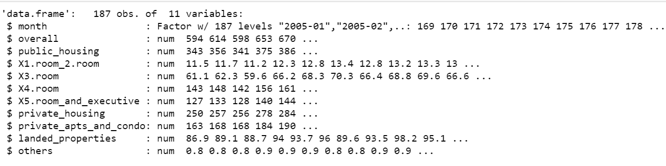
The ‘month’ column is originally in factor format with many levels. Let us convert it to a date type and select only relevant columns in the dataframe.
str(df)
# Change Factor to Date format
df$month <- paste(df$month, "01", sep="-")
# Select only relevant columns in a new dataframe
df$month <- as.Date(df$month,format="%Y-%m-%d")
df <- df %>% select(month,overall)
# Convert df to a tibble
df <- as_tibble(df)
class(df)
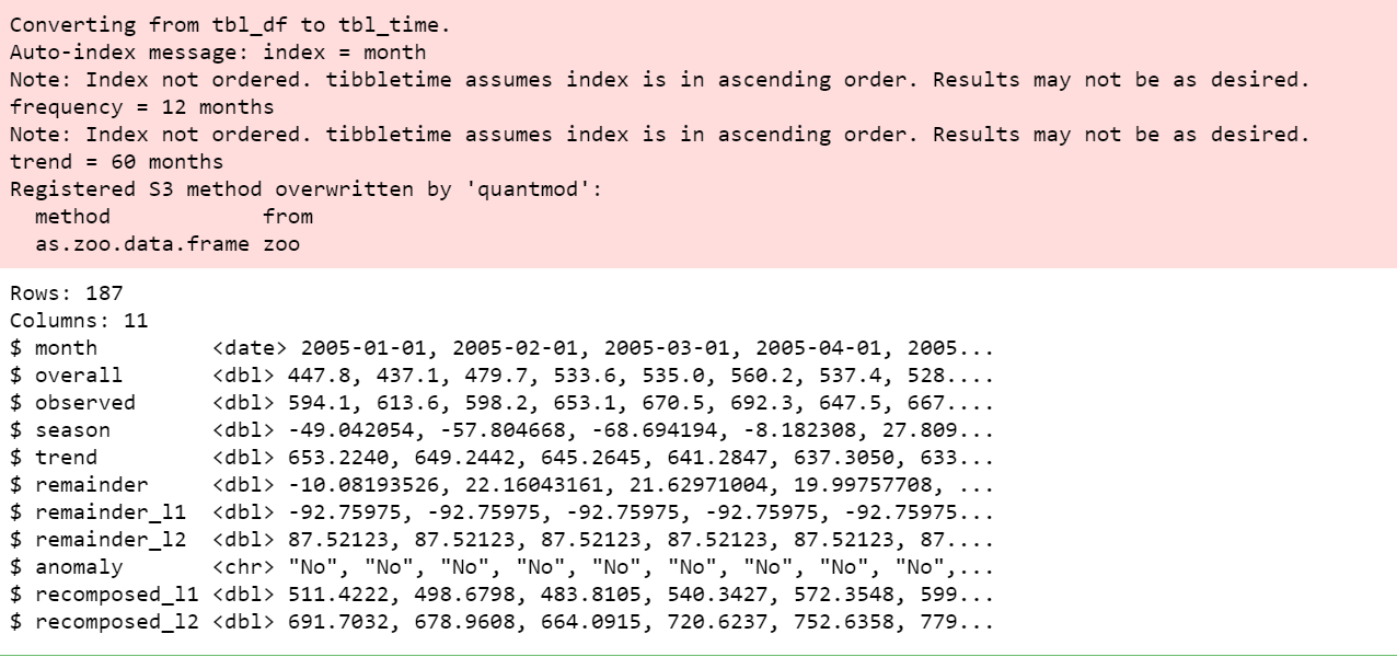
The R ‘anomalize’ package enables a workflow for detecting anomalies in data. The main functions are time_decompose(), anomalize(), and time_recompose().
df_anomalized <- df %>%
    time_decompose(overall, merge = TRUE) %>%
    anomalize(remainder) %>%
    time_recompose()
df_anomalized %>% glimpse()
We can then visualize the anomalies using the plot_anomalies() function.
df_anomalized %>% plot_anomalies(ncol = 3, alpha_dots = 0.75)
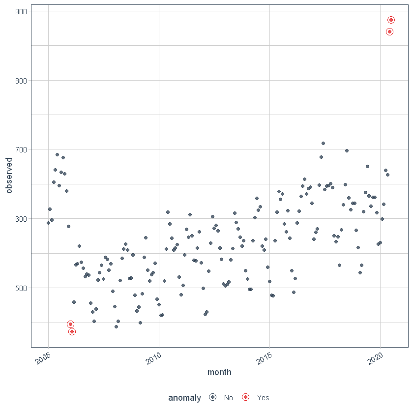
With anomalize, it’s simple to make adjustments because everything is done with a date or DateTime information so you can intuitively select increments by time spans that make sense (e.g. “5 minutes” or “1 month”).
First, notice that a frequency and a trend were automatically selected for us. This is by design. The arguments frequency = “auto” and trend = “auto” are the defaults. We can visualize this decomposition using plot_anomaly_decomposition().
p1 <- df_anomalized %>%
    plot_anomaly_decomposition() +
    ggtitle("Freq/Trend = 'auto'")
p1
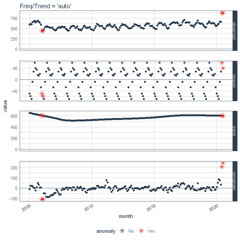
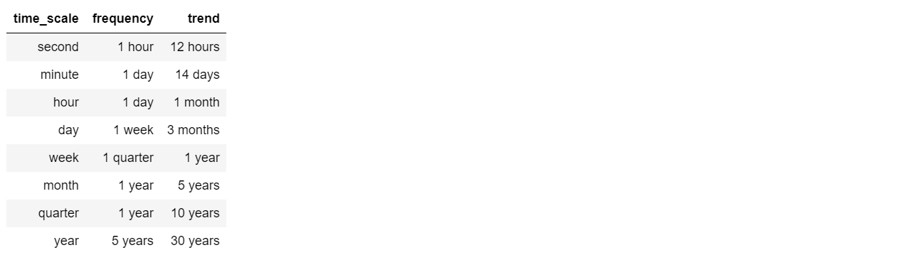
When “auto” is used, a get_time_scale_template() is used to determine the logical frequency and trend spans based on the scale of the data. You can uncover the logic:
get_time_scale_template()
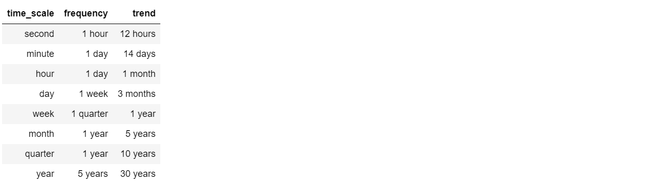
This implies that if the scale is 1 day (meaning the difference between each data point is 1 day), then the frequency will be 7 days (or 1 week) and the trend will be around 90 days (or 3 months). This logic can be easily adjusted in two ways: Local parameter adjustment & Global parameter adjustment.
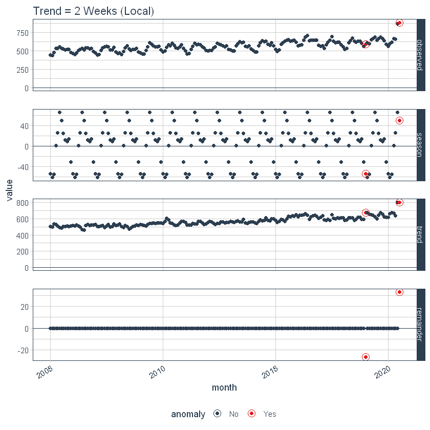
Local parameter adjustment is performed by tweaking the in-function parameters. Below we adjust trend = “2 weeks” which makes for a quite overfit trend.
p2 <- df %>%
    time_decompose(overall,
                   frequency = "auto",
                   trend     = "2 weeks") %>%
    anomalize(remainder) %>%
    plot_anomaly_decomposition() +
    ggtitle("Trend = 2 Weeks (Local)")
# Show plots
p1
p2

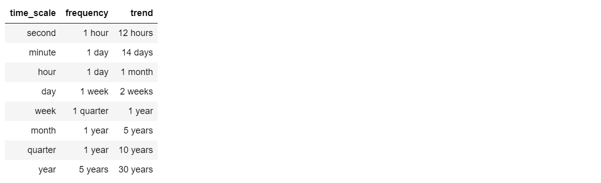
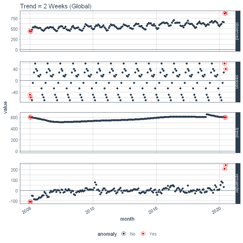
We can also adjust globally by using set_time_scale_template() to update the default template to one that we prefer. We’ll change the “3 month” trend to “2 weeks” for time scale = “day”. Use time_scale_template() to retrieve the time scale template that anomalize begins with, mutate() the trend field in the desired location, and use set_time_scale_template() to update the template in the global options. We can retrieve the updated template using get_time_scale_template() to verify the change has been executed properly.
time_scale_template() %>%
    mutate(trend = ifelse(time_scale == "day", "2 weeks", trend)) %>%
    set_time_scale_template()
get_time_scale_template()
p3 <- df %>%
    time_decompose(overall) %>%
    anomalize(remainder) %>%
    plot_anomaly_decomposition() +
    ggtitle("Trend = 2 Weeks (Global)")
p3
Let’s reset the time scale template defaults back to the original defaults.
time_scale_template() %>%
    set_time_scale_template()
# Verify the change
get_time_scale_template()
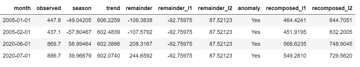
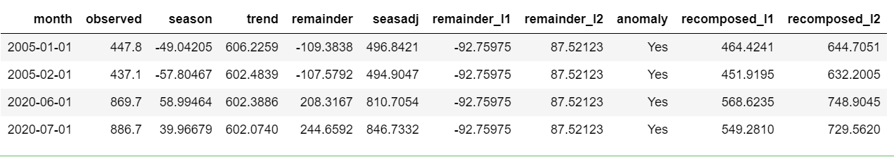
Now, we can extract the actual datapoints which are anomalies. For that, the following code can be run.
df %>%
  time_decompose(overall) %>%
  anomalize(remainder) %>%
  time_recompose() %>%
  filter(anomaly == 'Yes')
The alpha and max_anoms are the two parameters that control the anomalize() function. H
Alpha
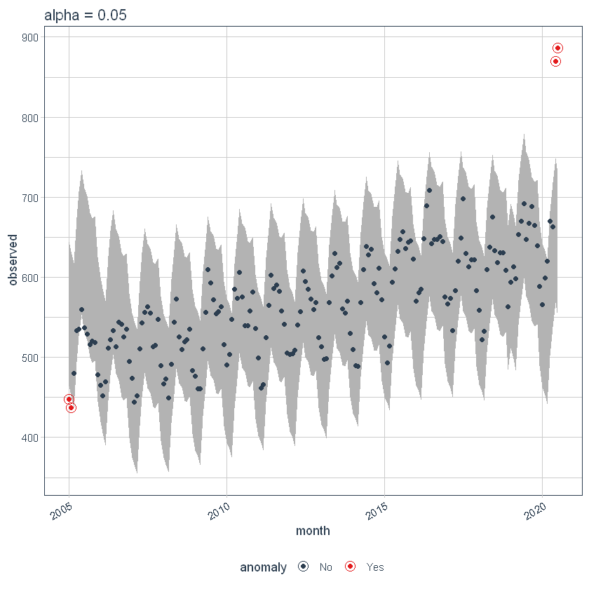
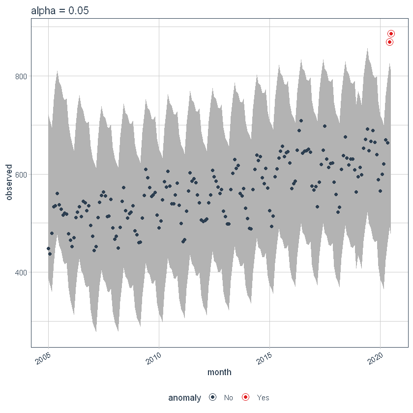
We can adjust alpha, which is set to 0.05 by default. By default, the bands just cover the outside of the range.
p4 <- df %>%
    time_decompose(overall) %>%
    anomalize(remainder, alpha = 0.05, max_anoms = 0.2) %>%
    time_recompose() %>%
    plot_anomalies(time_recomposed = TRUE) +
    ggtitle("alpha = 0.05")
#> frequency = 7 days
#> trend = 91 days
p4
If we decrease alpha, it increases the bands making it more difficult to be an outlier. Here, you can see that the bands have become twice big in size.
p5 <- df %>%
    time_decompose(overall) %>%
    anomalize(remainder, alpha = 0.025, max_anoms = 0.2) %>%
    time_recompose() %>%
    plot_anomalies(time_recomposed = TRUE) +
    ggtitle("alpha = 0.05")
#> frequency = 7 days
#> trend = 91 days
p5
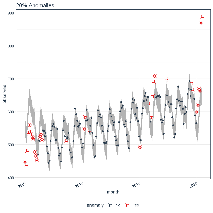
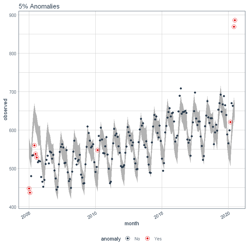
The max_anoms parameter is used to control the maximum percentage of data that can be an anomaly. Let’s adjust alpha = 0.3 so pretty much anything is an outlier. Now let’s try a comparison between max_anoms = 0.2 (20% anomalies allowed) and max_anoms = 0.05 (5% anomalies allowed).
p6 <- df %>%
    time_decompose(overall) %>%
    anomalize(remainder, alpha = 0.3, max_anoms = 0.2) %>%
    time_recompose() %>%
    plot_anomalies(time_recomposed = TRUE) +
    ggtitle("20% Anomalies")
#> frequency = 7 days
#> trend = 91 days
p7 <- df %>%
    time_decompose(overall) %>%
    anomalize(remainder, alpha = 0.3, max_anoms = 0.05) %>%
    time_recompose() %>%
    plot_anomalies(time_recomposed = TRUE) +
    ggtitle("5% Anomalies")
#> frequency = 7 days
#> trend = 91 days
p6
p7
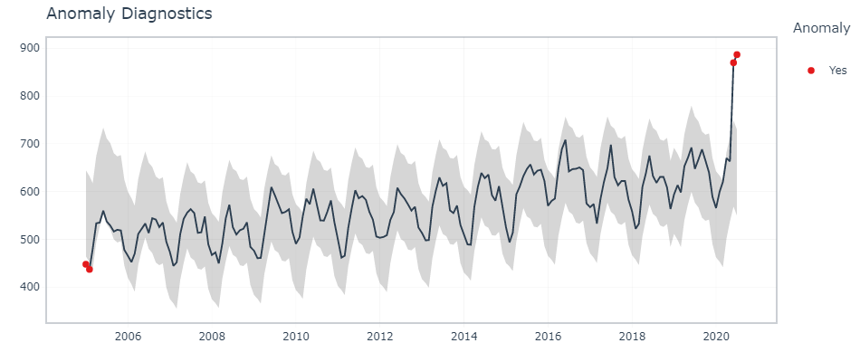
It is a ToolKit for working with Time Series in R, to plot, wrangle, and feature engineer time series data for forecasting and machine learning prediction.
Here, timetk’s plot_anomaly_diagnostics() function makes it possible to tweak some of the parameters on the fly.
df %>% timetk::plot_anomaly_diagnostics(month,overall, .facet_ncol = 2)
To find the exact data points that are anomalies, we use tk_anomaly_diagnostics() function.
df %>% timetk::tk_anomaly_diagnostics(month, overall) %>% filter(anomaly=='Yes')
In this article, we have seen some of the popular packages in R that can be used to identify and visualize anomalies in a time series. To offer some clarity of the anomaly detection techniques in R, we did a case study on a publicly available dataset. There are other methods to detect outliers and those can be explored too.
Lorem ipsum dolor sit amet, consectetur adipiscing elit,


