Misguiding Deep Neural Networks: Generalized Pixel Attack

This article was published as a part of the Data Science Blogathon.

Introduction

Recent advancements in machine learning and deep neural networks permitted us to resolve complicated realistic problems in images, video, text, genes, or many more. In the current scenario, deep learning-based approaches have overcome traditional image processing techniques. However, misguiding deep neural networks is easy with the help of just one-pixel alteration. That is, artificial perturbations on natural images can easily make DNN misclassify.

Before we go into the details, let us have a quick recap of the deep neural network.

Artificial Neural Network (ANN)

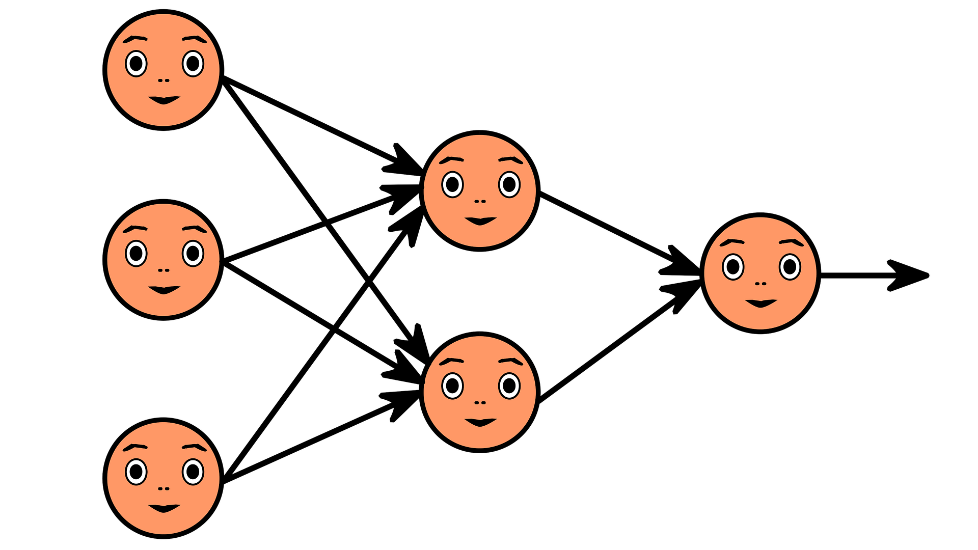
A neural network is a method that simulates the activity of the human brain and tries to mimic its decision-making capability. Superficially, it can be thought of as a network of an input layer, output layer, and hidden layer(s).

Each layer performs its specific task assigned to it and passes it to further processing to another one. This phenomenon is known as “feature hierarchy.” This feature comes quite handy when dealing with unlabeled or unstructured data.

Convolutional Neural Network (CNN)

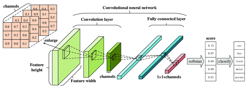
Convolutional Neural Network (CNN) or ConvNet for short, are the architectures that are mostly applied to images. The problem domain targeted by CNNs should not have spatial dependence. Another unique perspective of CNN is to get abstract features when input propagates from shallow to deeper layers.

Misguiding Deep Neural Networks by Adversarial Examples

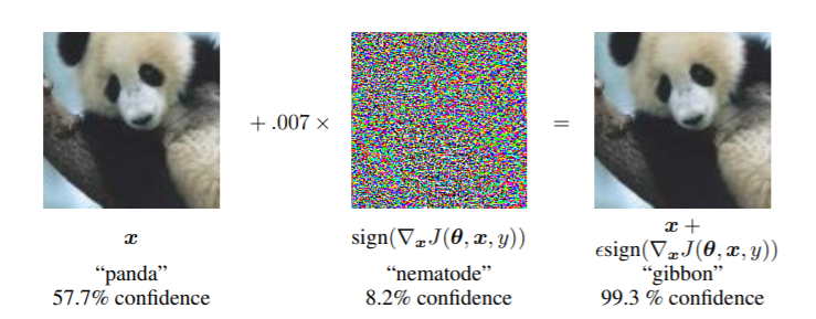
In 2015, people at Google and NYU affirmed that ConvNets could easily be fooled if the input is perturbated slightly. For example, our trained model recognizes the “Panda” with a confidence of 58%(approx.) while the same model classifies it as “Gibbon” with a much higher confidence of 99%. This is obviously an illusion for the network, which has been fooled by the noise thus inserted.

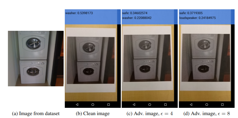
In 2017 again, a group of researchers at Google Brain and Ian J. Goodfellow showed that printed images, when captured through the camera and perturbated a slight, resulted in misclassification.

The umbrella term for all these scenarios is the Adversarial example.

The Threat

From the above examples, it is clear that the machine learning models are vulnerable to adversarial manipulations and result in misclassification. In particular, the misguiding of the output of Deep Neural Networks (DNN) can be easily done by adding relatively small perturbations to the input vector. The consideration for pixel attach as a threat involves:

1. Analysis of the natural images’ vicinity, that is, few pixel perturbations can be regarded as cutting the input space using low-dimensional slices.
2. A measure of perceptiveness is a straightforward way of mitigating the problem by limiting the number of modifications to as few as possible.

Mathematically, the problem can be posed as-

Let ‘f’ be the target image classifier which receives n-dimensional inputs,

x = (x₁, x₂, …, x_n), t

f_t(x) is the probability of correct class

The vector e(x) = (e₁,e₂, …, e_n) is an additive adversarial perturbation.

The limitation of maximum modification is L.

f_adv(x + e(x))

subject to e(x)<= L

The Attack: Targeted v/s Untargeted

An untargeted attack causes a model to misclassify an image to another class except for the original one. In contrast, a targeted attack causes a model to classify an image as a given target class. We want to perturb an image to maximize the probability of a class of our choosing.

The Defense

Increasing the Efficiency of the Differential Evolution algorithm such that the perturbation success rates should be improved and comparing the performance of Targeted and Untargeted attacks.

Differential Evolution

Differential evolution is a population-based optimization algorithm for solving complex multi-modal optimization. Differential Evolution

Moreover, it has mechanisms in the population selection phase that keep the diversity such that in practice, it is expected to efficiently find higher quality solutions than gradient-based solutions or even other kinds of EAs in specific during each iteration another set of candidate solutions (children) is generated according to the current population (fathers).

Why Differential Evolution?

There are three significant reasons to choose for Differential Evolution, viz.,

1. Higher probability of Finding Global Optima,
2. Require Less Information from Target System, and
3. Simplicity

In the context of a one-pixel attack, our input will be a flat vector of pixels, that is,

X=(x₁,y₁,r₁,g₁,b₁,x₂,y₂,r₂,g₂,b₂,…….)

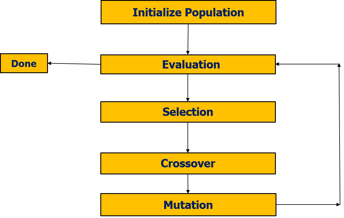
First, we generate a random population of n-perturbations

P=(x₁,x₂,….x_n)

Further, on each iteration, we calculate n new mutant children using the formula

X_i=x_r1+f(x_r2-x_r3)

such that

r1!=r2!=r3

The standard DE algorithm has three primary candidates for improvement: the crossover, the selection, and the mutation operator.

The selection has been unchanged from the original publication by Storn and Price to state-of-the-art variants of DE, making it less likely that improvements could significantly enhance the performance.

Crossover has a large effect on the search and is of particular importance when optimizing non-separable functions.

Mutation: Can be changed

The mutation operator has been among the most studied parts of the algorithm. Numerous variations published over the years provided all the required background knowledge about the population. It is just a matter of changing some variables or adding some terms to a linear equation. All this makes mutation the best step to improve.

The question then becomes which mutation operator to improve.

The DE/rand/1 operator seems to be the best choice because it is studied extensively, and the comparison of the implementation becomes effortless. Moreover, it would be interesting to see how effectively generating additional training data with dead pixels affects such attacks.

Whatever we put – 1 pixel, some error, noise, fuzz – or anything else, neural networks could give some false recognitions – entirely in an a-priory unpredictable way.

Conclusion

Adversarial examples prove that neural networks are fundamentally broken and can never lead to strong AI. The adversarial images for which only one pixel is altered are challenging to detect by humans.

References

1. Goodfellow, Ian J., Jonathon Shlens, and Christian Szegedy. “Explaining and harnessing adversarial examples.” arXiv preprint arXiv:1412.6572 (2014).
2. Kurakin, Alexey, Ian Goodfellow, and Samy Bengio. “Adversarial examples in the physical world.” arXiv preprint arXiv:1607.02533 (2016).
3. Moosavi-Dezfooli, S. M., Fawzi, A., Fawzi, O., Frossard, P., & Soatto, S. (2017). Analysis of universal adversarial perturbations. arXiv preprint arXiv:1705.09554.
4. Storn, Rainer, and Kenneth Price. “Differential evolution–a simple and efficient heuristic for global optimization over continuous spaces.” Journal of global optimization 11.4 (1997): 341-359.
5. Szegedy, C., Zaremba, W., Sutskever, I., Bruna, J., Erhan, D., Goodfellow, I., & Fergus, R. (2013). Intriguing properties of neural networks. arXiv preprint arXiv:1312.6199.
6. Wang, J., Sun, J., Zhang, P., & Wang, X. (2018). Detecting adversarial samples for deep neural networks through mutation testing. arXiv preprint arXiv:1805.05010.

Kopal Rastogi 16 Dec 2020