An Introduction to Hypothesis Testing
This article was published as a part of the Data Science Blogathon.
Introduction:
Many problems require that we decide whether to accept or reject some parameter. The statement is usually called a Hypothesis and the decision-making process about the hypothesis is called Hypothesis Testing. This is one of the most useful concepts of Statistical Inference since many types of decision problems can be formulated as hypothesis testing problems.
If an engineer has to decide based on sample data whether the true average lifetime of a certain kind of tire is at least 42,000 miles, or if an agronomist has to decide based on experiments whether one kind of fertilizer produces a higher yield of soybeans than another, and if a manufacturer of pharmaceutical products has to decide based on samples whether 90 percent of all patients given a new medication will recover from a certain disease or not, all of these problems can be translated into the language of statistical tests of hypotheses.
In the first case, we might say that the engineer has to test the hypothesis that θ, the parameter of an exponential population, is at least 42,000 while in the second case we might say that the agronomist has to decide whether μ1>μ2, where μ1 and μ2 are the means of two normal populations and in the third case we might say that the manufacturer has to decide whether θ, the parameter of a binomial population, equals 0.90. In each case it must be assumed, of course, that the chosen distribution correctly describes the experimental conditions; that is, the distribution provides the correct statistical model.
Table of Contents:
1. Hypothesis Testing
2. p-values and significance tests
3. Type I and Type II Errors
4. Power
5. Error probabilities and ∝
6. Summary
1. Hypothesis Testing:
Suppose we want to show that one kind of ore has a higher percentage content of uranium than another kind of ore, we might formulate the hypothesis that the two percentages are the same; and if we want to show that there is greater variability in the quality of one product than there is in the quality of another, we might formulate the hypothesis that there is no difference; that is, σ1 = σ2. Given the assumptions of “no difference,” hypotheses such as these led to the term null hypothesis. Symbolically, we shall use the symbol H0 for the null hypothesis that we want to test and H1 or Ha for the alternative hypothesis.
H0: This is the hypothesis where things are happening as expected i.e. “ no difference”
It will often have a statement of equality where the population parameter is equal to a value where the value is what people were kind of assuming all along.
Ha: This is a claim where if you have evidence to back up that claim, that would be new news.
Example: The National Sleep Foundation recommends that teenagers aged 14 to 17 years old need to get at least 8 hours of sleep per night for proper health and wellness.
A statistics class at a large high school suspects that students at their school are getting less than 8 hours of sleep on average. To test their theory, they randomly sample 42 of these students and ask them how many hours of sleep they get per night. The mean from the sample is 7.5 hours. Write Null and Alternative hypothesis.
Ho: µ ≥ 8 hours
Ha: µ<8 hours
where, µ = Population mean & not sample mean
2. P – values and Significance tests
Rather than having formal rules for when to reject the null hypothesis, one can report the evidence against the null hypothesis. This is done by reporting the significance level of the test, also known as the P-value. The P-value is computed under the assumption that the null hypothesis is true and is the probability of seeing data that are as extreme or more extreme than those that were observed. In other words, it is the level at which the testing would just barely be rejected.
Suppose we have a website that has a white background and the average engagement on the website by any user is around 20 minutes. Now we are proposing a new website with a yellow background that might increase the average engagement by any user to more than 20 minutes. So, we state the null and alternate hypothesis as:
1. H0: µ = 20 min after the change
Ha: µ > 20 min after the change
2. Significance Level : ∝ = 0.05
Now we are going to take a sample of people visiting this new yellow background website and we are going to calculate statistics i.e. sample mean, and we are going to say, hey, if we assume that the null hypothesis is true, what is the probability of getting a sample with the statistics that we get? And if that probability is lower than our significance level (i.e. less than 5%), then we reject the null hypothesis and say that we have evidence for the alternative. However, if the probability of getting the statistics for that sample is at the significance level or higher, then we say, “Hey, we can’t reject the null hypothesis and we aren’t able to have evidence for the alternative”.
3. Take a sample: n = 100
x̅ = 25 min
4. p-value (Probability value): It is the probability of getting a statistic at least this far away from the mean if we were to assume that the null hypothesis is true.
P-value : P(x̅ ≥ 25 min | H0 is true) This is a conditional probability
5. If P-value < ∝ —-> Reject H0
P-value ≥ ∝ —-> Do not reject H0
Note: Significance level (∝) should be set ahead of time when we do our experiment due to ethical issues as it might be tempting to set ∝ as per our result in order to reject H0
In practice, we should make our hypothesis and set our significance level ∝ before we collect or see any data which we choose depends on the consequences of various errors.
3. Type I and Type II Errors :
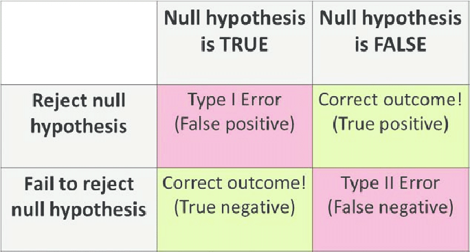
The Probability of getting a type I error is the significance level because if our null hypothesis is true, let’s say that our significance level is 5%. Well, 5% of the time, even if our null hypothesis is true, we are going to get a statistic that’s going to make you reject the null hypothesis. So, one way to think about the probability of a Type I error is our significance level.
Type I error: Rejecting null hypothesis H0 even though it is true. Because it is so unlikely to get a statistic like that assuming the null hypothesis is true, we decide to reject the null hypothesis.
4. Power
This is the probability that you are doing the right thing when the null hypothesis is not true i.e. we should reject the null hypothesis if it’s not true.
Hence, Power = P(rejecting H0 | H0 is false)
= 1- P(not rejecting H0 | H0 is false) —> This is called Type II Error
= P( not making a Type II Error )
Example: Let H0: µ = µ1
Ha: µ ≠ µ1
Note:
1. If we increase ∝( significance level ), power increases i.e. ∝⇧ —> Power ⇧
But it also increases type I error i.e. P( type I error) ⇧
2. If we increase n (sample size), power increases i.e. n ⇧ —> Power ⇧
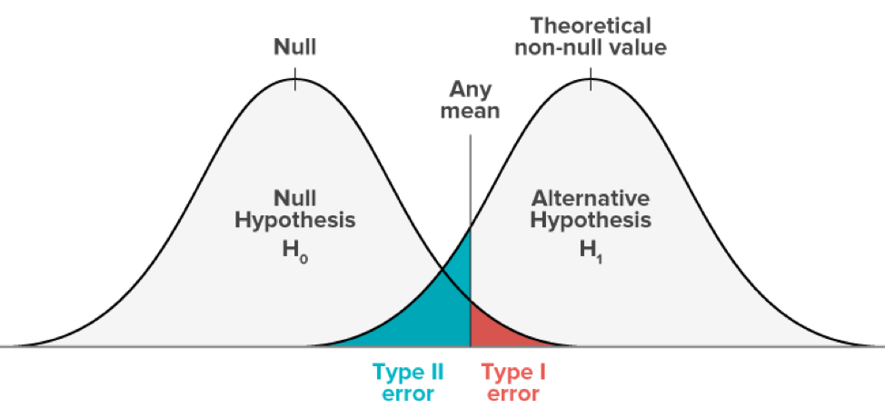
This in general is always a good thing. Increasing n causes narrower curve & overlapping between 2 curves reduces.
3. Less variability (i.e. σ2 or σ) in data set also makes sampling distribution narrower so it increases Power. If the true parameter is further away than what the null hypothesis is saying then power increases.
5. Error probabilities and ∝ :
1. A Type I error is when we reject a true null hypothesis. Lower values of ∝ making it harder to reject the null hypothesis, so choosing lower values ∝ can reduce the probability of Type I error. The consequence here is that if the null hypothesis is false, it may be difficult to reject using lower values ∝. So using lower values ∝ can increase the probability of a Type II error.
2. A Type II error is when we fail to reject a false null hypothesis. Higher values of ∝ making it easier to reject the null hypothesis, so choosing higher values ∝ can reduce the probability of a Type II error. The consequence here is that if the null hypothesis is true, increasing ∝ makes it more likely that we commit a Type I error (rejecting a true null hypothesis).
6. Summary
Hypothesis Testing can be summarized using the following steps:
1. Formulate H0 and H1, and specify α.
2. Using the sampling distribution of an appropriate test statistic, determine a critical region of size α.
3. Determine the value of the test statistic from the sample data.
4. Check whether the value of the test statistic falls into the critical region and, accordingly, reject the null hypothesis, or reserve judgment. (Note that we do not accept the null hypothesis because β, the probability of false acceptance, is not specified in a test of significance.)
The media shown in this article are not owned by Analytics Vidhya and is used at the Author’s discretion.


