Inferential Statistics – Sampling Distribution, Central Limit Theorem and Confidence Interval
This article was published as a part of the Data Science Blogathon.
Introduction
The field of statistics consists of methods for describing and modeling variability and for making decisions when variability is present. In inferential statistics, we usually want to make a decision about some population. The population refers to the collection of measurements on all elements of a universe about which we wish to draw conclusions or make decisions.
In most application of statistics, the available data result from a sample of units selected from a universe of interest.
Table of Content
1. Sampling Distribution
2. Sampling distribution of sample proportion
3. Central Limit Theorem
4. Confidence Interval
5. Conditions for inference on a proportion and mean
1. Sampling Distribution
Suppose we have a population with population parameters (µ,σ). We may not know the population parameters or it may not even be easy to find the population parameters. So, we try to estimate a population parameter by taking a sample of size n and calculate a statistic that is used to estimate the parameter.
If we were to take a random sample of size n again and then we were to calculate the statistic again, we could very well get a different value.
Hence, what is the distribution of the values that we could get for the statistic? What is the frequency with which I can get different values for the statistic that is trying to estimate the population parameter? And that distribution is what a sampling distribution is.
Example
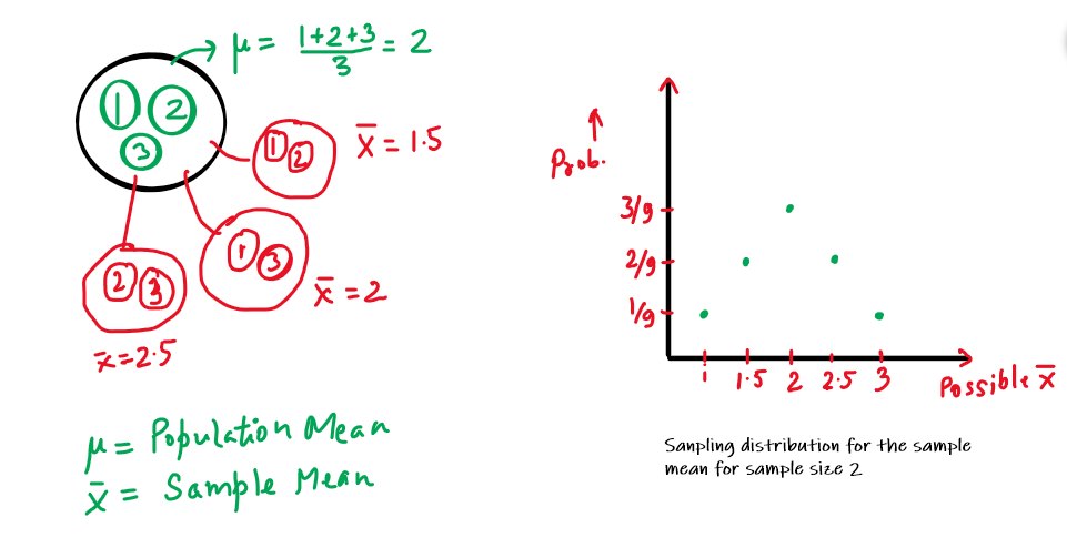
Suppose we have a population containing three numbers – 1,2 and 3. The mean of the population (denoted by µ) will be (1+2+3)/3 i.e. 2. Now, we take random samples of size 2 from the population and report the sample statistic i.e x̅ of the sample every time.
| #’s picked | x̅ |
| 1,1 | 1 |
| 1,2 | 1.5 |
| 1,3 | 2 |
| 2,1 | 1.5 |
| 2,2 | 2 |
| 2,3 | 2.5 |
| 3,1 | 2 |
| 3,2 | 2.5 |
| 3,3 | 3 |
2. Sampling distribution of sample proportion
Suppose we have a big bowl containing 10,000 different colored balls having 60% of the yellow-colored balls. Then the population parameter is p = 0.6. Let Y be a random variable taking value 1 when we get a yellow ball from the bowl and 0 when we get a different coloured ball. Clearly, Y follows Bernoulli distribution. The mean and standard deviation of Y is 0.6 and 0.49.
Let X be another random variable denoting the sum of 10 independent Bernoulli trails. The mean and variance of X is 10×0.6 = 6 and standard deviation is 1.55
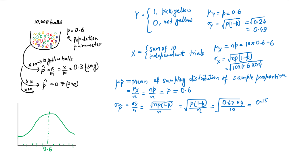
Note that the sampling distribution of sample proportion is approximately normal in shape if np >= 10 and n(1-p) >= 10.
3. Central Limit Theorem
The Central Limit Theorem(CLT) states that the distribution of sample means approximates a normal distribution as the sample size becomes larger, assuming all the samples are identical in size, and regardless of the population distribution shape i.e. when mean of a sampling distribution of a random variable (may be any random variable, not necessarily binomial random variable that we have taken in the previous example) is plotted on a frequency distribution curve, it approximates a normal distribution

A few things to note:
1. CLT states that the distribution of sample means approximates a normal distribution as the sample size gets larger
2. Sample size >= 30 are considered sufficient for the CLT to hold
3.
4. Confidence Interval
Suppose there are 100,000 voters and there are 2 candidates A and B competing in the election. We want to find out the likelihood that candidate A wins the election.
Since the population proportion i.e. proportion that supports A is unknown, in order to estimate the population proportion, we take many samples from the population (say sample size, n = 100) and calculate the sample proportion for each sample.
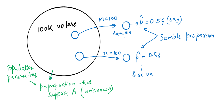
Since our sample size is so much smaller than the population(it’s way less then 10%), we can assume that each person we are asking about their preference between A and B is approximately independent. We actually don’t know the what the actual population parameter is (i.e. p).
So, for the 1st case, i.e. n = 100 and p-hat = 0.54, we could have got all sorts of outcomes. Sample proportion p-hat = 0.54 may have been above ‘p’ (population parameter) or below p. We have this uncertainty because we actually don’t know what the real population proportion(parameter) is.
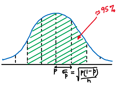
Now, we are interested in – What is the probability that p-hat = 0.54 is within 2 standard deviation of p? (i.e. 95%) i.e. If I take a sample size of 100 and I calculate sample proportion, what is the probability that I am going to be within 2 standard deviation 95% of the time.
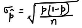
Since the p is not known, standard deviation of the sample proportion can not be calculated. Instead, we will calculate Standard Error of Sample proportion
So, for 95% confidence,
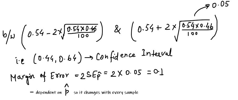
It will produce intervals (and intervals won’t always be the same as it is dependent on our sample proportion) which will include true proportion i.e. population proportion ‘p’ 95% of the time.
If we wanted to tighten up the intervals, i.e. we have to lower our margin of error i.e. we have to increase n(sample size) as Standard Error is inversely proportional to n.
So, the question that we answer with the confidence interval is: For any given estimate (sample) how confident are we that the certain range around that sample actually contains the true population proportion?
Note:
1. The confidence ‘level’ refers to the long term success rate of the method i.e. how often this type of interval will capture the parameter of interest.
2. A specific confidence interval gives a range of plausible values for the parameter of interest.
3. A larger margin of error produces a wider confidence interval that is more likely to contain the parameter of interest(increased confidence)
4. Increasing the confidence will increase the margin of error resulting in a wider interval.
Example:
Suppose a baseball coach was curious about the true mean speed of fastball pitches in his league. The coach recorded the speed in km/hr of each fastball in a random sample of 100 pitches and constructed a 95% confidence interval for the mean speed. The resulting interval was (110,120). Can we say there is a 95% chance that the true mean is between 110 and 120 km/hr?
In such a case, we would not say there is a 95% chance that this specific interval contains the true mean because it implies that the mean may be within this interval, or it may be somewhere else. This phrasing makes it seem as if the population mean is variable, but it’s not. This interval either captured the mean or didn’t. Intervals change from sample to sample, but the population parameter we are trying to capture does not.
It’s safer to say that we are 95% confident that this interval captured the mean, since this phrasing more closely agrees with the long-term capture rate of confidence levels.
5. Conditions for inference on a proportion and mean
1. Random Condition : Random samples give us unbiased data from a population. When samples aren’t randomly selected, the data usually has some form of bias, so using data that wasn’t randomly selected to make inference about its population can be risky.
2. The Normal Condition : The sampling distribution of p-hat is approx. normal as long as the expected number of successes and failures are both at least 10. This happens when our sample size n is reasonably large.
So, expected success : np >= 10 Expected failures : n(1-p) >= 10
If we are building a confidence interval, we don’t have a value of p to plug in, so we instead count the observed number of successes and failures in the sample data to make sure they are both at least 10.
3. The Independence condition : To use the formula for standard deviation of p-hat, we need individual observations to be independent. When we are sampling without replacement, individual observations aren’t technically independent since removing each item changes the population.
But the 10% condition says that if we sample 10% or less of the population, we can treat individual observations doesn’t significantly change the population as we sample. This allows us to use the formula for standard deviation of p-hat.
In a significance test, we use the sample size n and the hypothesized value of p.
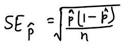
If we are building a confidence interval for p, we don’t actually know what p is, so we substitute p-hat as an estimate for p. When we do this, we call it the standard error of p-hat to distinguish it from the standard deviation. So our formula for standard error of p-hat is
The media shown in this article are not owned by Analytics Vidhya and is used at the Author’s discretion.


Nice.. this help me so much....
Very useful information..