New Approach for Regression Analysis – RANSAC and MLESAC
This article was published as a part of the Data Science Blogathon.
Introduction
The aim of this article is to obtain the best possible results for the analysis of real data points, in general, but here as an example, for a fictive Engine Retardation.
The results of any of these measurements can be misleading, maybe because of these:
- A low magnitude cause inaccurate measurements.
- The presence of measurement dips that result in significant variation in the calculated value over the period of a scan.
- The results can be influenced by data spikes.
- Unintentional generation, propagation, and reception of electromagnetic energy among an electromagnetic device (engine, generator, etc.) with reference to unwanted effects (electromagnetic interference, or EMI) that such energy may induce.
- Inaccurate measurement devices with too high deviations.
All these effects can have a massive influence on the accuracy of a measurement. Most of the effects cannot be resolved without going further but can be covered with the help of the algorithm described below.
Here in this article, these misleading data points are simply called outliers.
To calculate the straight regression line from fictive measurement points (called engine retardation), a floating Linear Least Squares Fit (LLSF) algorithm is used. The LLSF estimation is a good method if assumptions are met to obtain regression weights when analyzing the engine data. However, if the data does not satisfy some of these assumptions, then sample estimates and results can be misleading. Especially, outliers violate the assumption of normally distributed residuals in the least-squares regression. The fact of outlying engine power data points (engine dips), in both the direction of the dependent (y-axis) and independent variables (x-axis/timestamp), to the least-squares regression is that they can have a strong adverse effect on the estimate and they may remain unnoticed. Therefore, techniques like RANSAC (Random Sample Consensus) that are able to cope with these problems or to detect outliers (bad) and inliers (good) have been developed by scientists and implemented into SimplexNumerica.
Robust consensus algorithms like RANSAC are important methods for analyzing data that are contaminated with outliers. It can be used to detect outliers and to provide resistant results in the presence of outliers.
A new approach based on the Maximum Likelihood Estimator Sample Consensus (MLESAC[1]) and Random Sample Consensus (RANSAC[2]) for an improved Engine Retardation measurement routine inside the device is described for robustly estimating floating linear regression relations from engine PowerPoint correspondences. The method comprises two parts. The first is a new robust estimator MLESAC that is a generalization of the RANSAC estimator. It adopts the same sampling strategy as RANSAC to generate putative solutions but chooses the solution that maximizes the likelihood rather than just the number of inliers. The second part of the algorithm is a general-purpose method for automatically parameterizing these relations, using the output of MLESAC.
Quintessence:
The new approach should be an established algorithm for maximum-likelihood estimation by random sampling consensus, devised for Engine Retardation measurement to avoid the influence of the above-described misleading results.
Random Sample Consensus (RANSAC)
The Random Sample Consensus (RANSAC) algorithm proposed by Fischler and Bolles[3] is a general parameter estimation approach designed to cope with a large proportion of outliers in the input data. Its basic operations are:
- Select sample set
- Compute model
- Compute and count inliers
- Repeat until sufficiently confident
Step ( i )
Step ( i + j )
Step n (result)
Result
The RANSAC steps in more details are[4]:
- Select randomly the minimum number of points required to determine the model parameters.
- Solve for the parameters of the model.
- Determine how many points from the set of all points fit with a predefined tolerance.
- If the fraction of the number of inliers over the total number of points in the set exceeds a predefined threshold, re-estimate the model parameters using all the identified inliers and terminate.
- Otherwise, repeat steps 1 through 4 (maximum of N times).
Briefly, RANSAC uniformly at random selects a subset of data samples and uses it to estimate model parameters. Then it determines the samples that are within an error tolerance of the generated model.
These samples are considered as agreed with the generated model and called as consensus set of the chosen data samples. Here, the data samples in the consensus as behaved as inliers and the rest as outliers by RANSAC. If the count of the samples in the consensus is high enough, it trains the final model of the consensus by using them.
It repeats this process for a number of iterations and returns the model that has the smallest average error among the generated models. As a randomized algorithm, RANSAC does not guarantee to find the optimal parametric model with respect to the inliers. However, the probability of reaching the optimal solution can be kept over a lower bound by assigning suitable values to algorithm parameters.
Maximum Likelihood Estimator Sample Consensus (MLESAC)
This chapter describes in a simple and concise way the robust estimator, MLESAC[5], which can be used for calculation instead of the floating regression algorithm LLSF.
In particular, MLESAC is well suited to estimating the Engine Retardation trend or more general, it manifolds the engine’s power data to timestamp miss relation in Engine Retardation measurement because of the fact that the timestamp is set maybe inaccurately inside the internal clock of the measurement device.
Technical descriptions and own tests have shown that the RANSAC algorithm has been proven very successful for robust estimation, but with the robust negative log-likelihood function having been defined as the quantity to be minimized it becomes apparent that RANSAC can be improved on. One of the problems with RANSAC is that if the threshold for considering inliers is set too high then the robust estimate can be very poor and the slope of the regression line goes wrong.
As an improvement over RANSAC, MLESAC has a better estimate for the elimination of noise dips for instance influenced by neighborhood machines. The minimal set point, initially selected by MLESAC, is known to provide a good estimate of the data relation. Hence, the initial estimate of the point basis provided by MLESAC is quite close to the true solution and consequently, the nonlinear minimization typically avoids local minima. Then the parameterization of the algorithm is consistent, which means that during the gradient descent phase-only data relations that might actually arise are searched for. It has been observed that the MLESAC method of robust fitting is good for initializing the parameter estimation when the data are corrupted by outliers. In this case, there are just two classes to which a datum might belong, inliers or outliers.
Torr and Zisserman have shown that the implementation of MLESAC yields a modest to hefty benefit to all robust estimations with absolutely no additional computational burden. In addition, the definition of the maximum likelihood error allows it to suggest a further improvement against RANSAC. As the aim is to minimize the negative log-likelihood of the data it makes sense to use this as the score for each of the random samples.
After MLESAC is applied, nonlinear minimization is conducted using the method described in Gill and Murray[6], which is a modification of the Gauss-Newton method. All the points are included in the minimization, but the effect of outliers is removed as the robust function places a ceiling on the value of their errors, unless the parameters move during the iterated search to a value where that correspondence might be reclassified as an inliers. This scheme allows outliers to be reclassed as inliers during the minimization itself without incurring additional computational complexity. This has the advantage of reducing the number of false classifications, which might arise by classifying the correspondences at too early a stage.
Evaluation of Samples
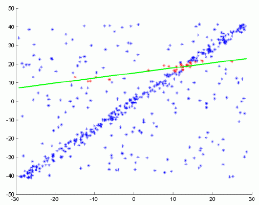
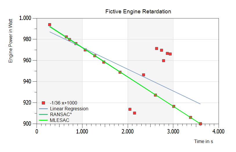
To show some results of the new SimplexNumerica algorithms, the following samples are evaluated. All have simulated data randomized around the slope f(x) = m x + b, m = 1/36, b = 1000. The inverse value of the difference quotient (m) is equal to the rundown time in (s/W). The next figure shows two outliers down under the theoretical graph – fitted by RANSAC (green line).
Example with two outliers:
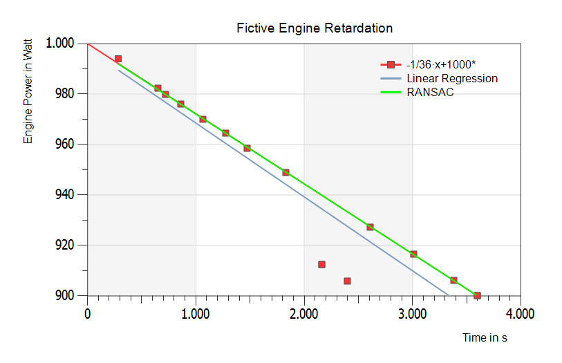
The above figure shows the theoretical regression line f(x) = m x + b in red, the floating Linear Least Squares Fit (LLSF or Linear Regression) in blue, and the RANSAC line in green (on top of the red one).
Result
RANSAC and theoretical line are nearly equal. The Linear Regression line drops away. The next figure has more outliers and some inliers to direct the real engine power.
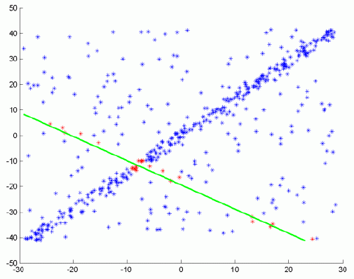
The above figure has more outliers and some inliers to direct the real rundown slope. The Linear Regression (blue line) goes away again. RANSAC (dark green line) does not find the right way. But finally: MLESAC (bright green line) shows the right fit to the real inliers.
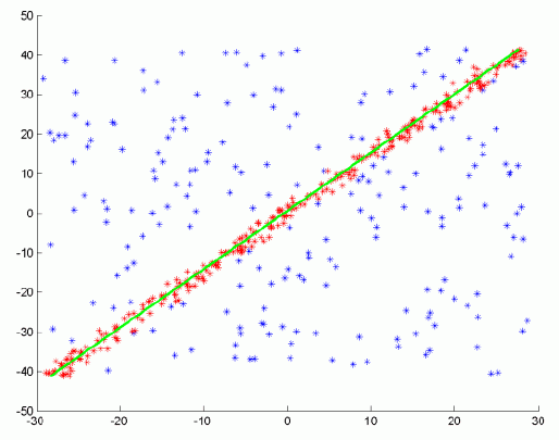
The above figure is similar to the previous one, but the additional two outliers have more distance down under the real line as in the figure before. Result: RANSAC and MLESAC are fitting best and lying on the same line.
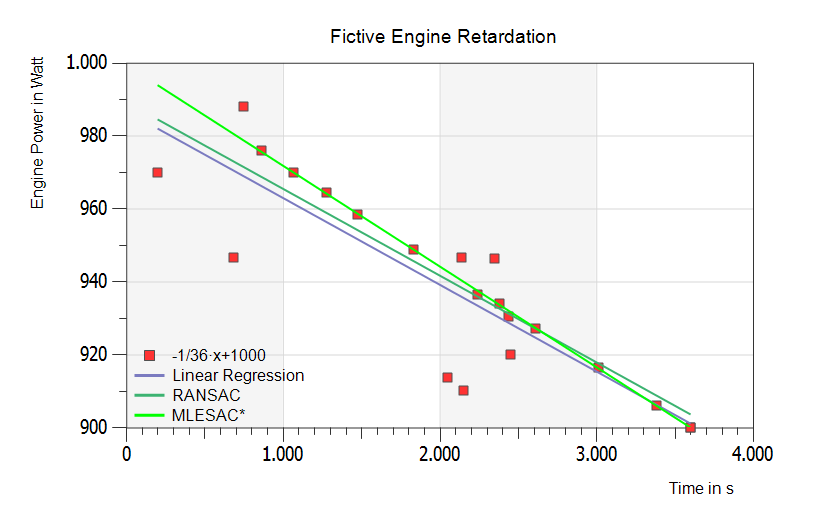
The bright green MLESAC regression line y(x) = m x + b yields best with the following statistical data:
- Estimated Slope: m = -0.0276023 à 1 / 0.0276023 ~ 36 s/W
- Estimated Y-axis Intercept: b = 999.415 ~ 1000 W
- Maximum number of iterations: n = 1000
- Distance to the model threshold: d = 0.001
- Probability of at least one SampleData free from outliers = 99 %
Conclusion
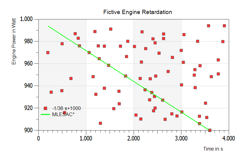
Also under these extremely difficult-to-identifying conditions, the MLESAC algorithm can accurately predict the right offset and slope of the Engine Power line with the result that the Engine Retardation is now the right one.
Lastly, extreme outliers far from realism – but still the right regression line:
[1] The MLESAC here represents an implementation of the MLESAC (Maximum Likelihood Estimator Sample Consensus) algorithm, as described in: “MLESAC: A new robust estimator with application to estimating image geometry”, P.H.S. Torr and A. Zisserman, Computer Vision and Image Understanding, vol 78, 2000.
[2] http://de.wikipedia.org/wiki/RANSAC-Algorithmus
[3] Martin A. Fischler and Robert C. Bolles (June 1981). “Random Sample Consensus: A Paradigm for Model Fitting with Applications to Image Analysis and Automated Cartography”. Comm. of the ACM 24 (6): 381–395. doi:10.1145/358669.358692
[4] From: Overview of the RANSAC Algorithm, Konstantinos G. Derpanis, [email protected], Version 1.2, May 13, 2010.
Or: M.A. Fischler and R.C. Bolles. Random sample consensus: A paradigm for model fitting with applications to image analysis and automated cartography. Communications of the ACM, 24(6):381–395, 1981.
[5] MLESAC: A New Robust Estimator with Application to Estimating Image Geometry P. H. S. Torr
Microsoft Research Ltd., St George House, I Guildhall St, Cambridge CB2 3NH, United Kingdom and A. Zisserman
Robotics Research Group, Department of Engineering Science, Oxford University, OX1 3PJ, United Kingdom
[6] P. E. Gill and W. Murray, Algorithms for the solution of the nonlinear least-squares problem, SIAM J. Numer.
Anal. 15(5), 1978, 977–992.
The media shown in this article are not owned by Analytics Vidhya and is used at the Author’s discretion.


