Introduction to K-Fold Cross-Validation in R

Prerequisites: Basic R programming language and basic classification knowledge
K-fold cross-validation is one of the most commonly used model evaluation methods. Even though this is not as popular as the validation set approach, it can give us a better insight into our data and model.
While the validation set approach is working by splitting the dataset once, the k-Fold is doing it five or ten times. Imagine you are doing the validation set approach ten times using a different group of data.otherother
Let’s say that we have 100 rows of data. We randomly divide them into ten groups of folds. Each fold will consist of around 10 rows of data. The first fold is going to be used as the validation set, and the rest is for the training set. Then we train our model using this dataset and calculate the accuracy or loss. We then repeat this process but using a different fold for the validation set. See the image below.

K-Fold cross-validation. Image by the author
Let’s jump into code
Libraries that we use are these two:
library(tidyverse)
library(caret)
The data used here is heart-disease data from UCI which can be downloaded on Kaggle. You can also use any classification data for this experiment.
data <- read.csv("../input/heart-disease-uci/heart.csv")
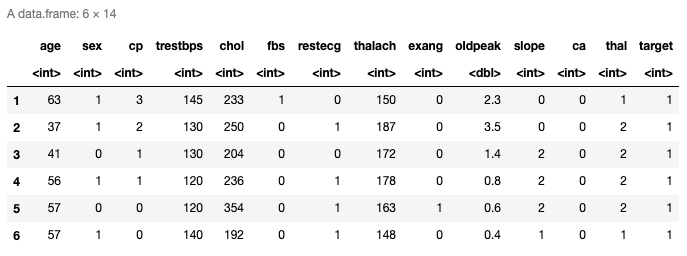
head(data)
Here are the top six rows of the loaded data. It has thirteen predictors and the last column is the response variable. You can also check the last rows using tail() function.
The Data Distribution
Here we want to confirm that the distribution between the two label data is not too much different. Because imbalanced datasets can lead to imbalanced accuracy. This means that your model will always predict towards one label only, either it will always predict 0 or 1.
hist(data$target,col="coral")
prop.table(table(data$target))
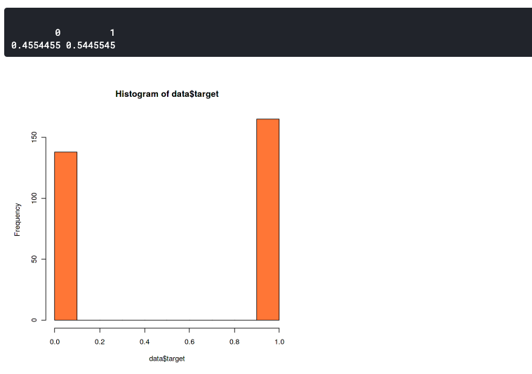
This plot shows that our dataset slightly imbalanced but still good enough. It has a 46:54 ratio. You should start to worry if your dataset has more than 60% of the data in one class. In that case, you can use SMOTE to handle an imbalanced dataset.
The k-Fold
set.seed(100)
trctrl <- trainControl(method = "cv", number = 10, savePredictions=TRUE)
nb_fit <- train(factor(target) ~., data = data, method = "naive_bayes", trControl=trctrl, tuneLength = 0)
nb_fit
The first line is to set the seed of the pseudo-random so that the same result can be reproduced. You can use any number for the seed value.
Next, we can set the k-Fold setting in trainControl() function. Set the method parameter to “cv” and number parameter to 10. It means that we set the cross-validation with ten folds. We can set the number of the fold with any number, but the most common way is to set it to five or ten.
The train() function is used to determine the method we use. Here we use the Naive Bayes method and we set the tuneLength to zero because we focus on evaluating the method on each fold. We can also set the tuneLength if we want to do the parameter tuning during the cross-validation. For example, if we use the K-NN method, and we want to analyze how many K is the best for our model.
You can see the supported method in R documentation.
Please keep in mind that k-Fold cross-validation could take a while because it runs the training process ten times.
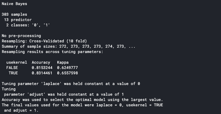
It will print the detail to the console once it is finished. The accuracy shown in the console is the average accuracy from all the training folds. We can see that our model has an 83% average accuracy.
Unfold the k-Fold
We can determine that our model is performing well on each fold by looking at each fold’s accuracy. In order to do this, make sure to set the savePredictions parameter to TRUE in the trainControl() function.
pred <- nb_fit$pred
pred$equal <- ifelse(pred$pred == pred$obs, 1,0)
eachfold <- pred %>%
group_by(Resample) %>%
summarise_at(vars(equal),
list(Accuracy = mean))
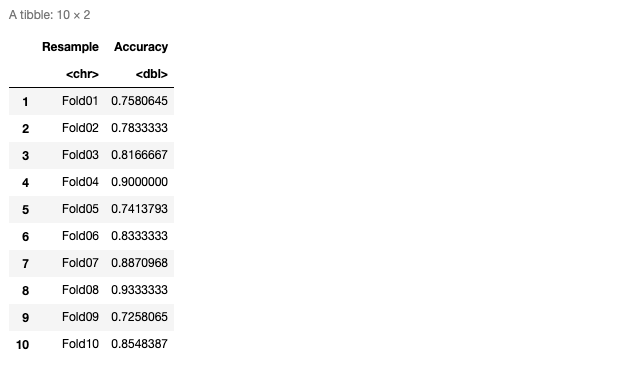
eachfold
Here’s the table of accuracy on each fold
We can also plot it to the graph so it’ll be easier to analyze. In this case, we used the boxplot to represent our accuracies.
ggplot(data=eachfold, aes(x=Resample, y=Accuracy, group=1)) +
geom_boxplot(color="maroon") +
geom_point() +
theme_minimal()
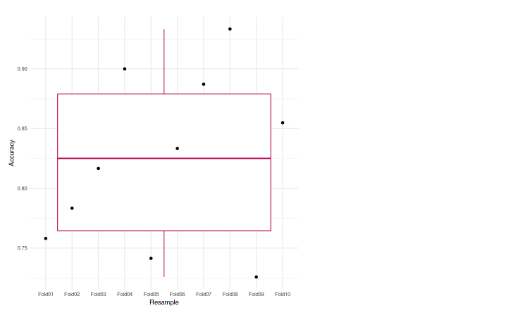
We can see that each of the folds achieves an accuracy that is not much different from one another. The lowest accuracy is 72.58%, and also in the boxplot, we do not see any outliers. Meaning that our model was performing well across the k-fold cross-validation.
What’s next
- Try a different number of folds
- Do a parameter tuning
- Use other datasets and methods
Short Author Bio
My name is Muhammad Arnaldo, a machine learning and data science enthusiast. Currently a master’s student of computer science in Indonesia.
The media shown in this article are not owned by Analytics Vidhya and is used at the Author’s discretion.


Keep your beneficial research up! It must be great to share good innovation and thoughts for those who need it.
Keep your good work up!