Beginner’s Guide to Low Variance Filter and its Implementation
Introduction
In the previous article, Beginner’s Guide to Missing Value Ratio and its Implementation, we saw a feature selection technique- Missing Value Ratio. In this article, we’re going to cover another technique of feature selection known as Low variance Filter.
Note: If you are more interested in learning concepts in an Audio-Visual format, We have this entire article explained in the video below. If not, you may continue reading.
Let’s take up the same dataset we saw earlier, where we want to predict the count of bikes that have been rented-
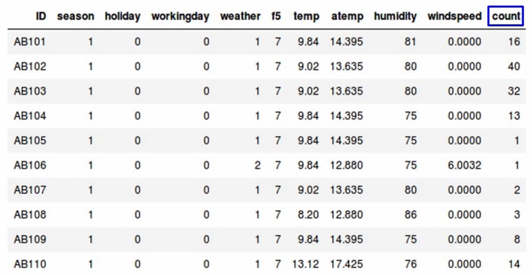
Now let’s assume there are no missing values in this data. If you look at the f5 variable, all the values you’ll notice are the same-
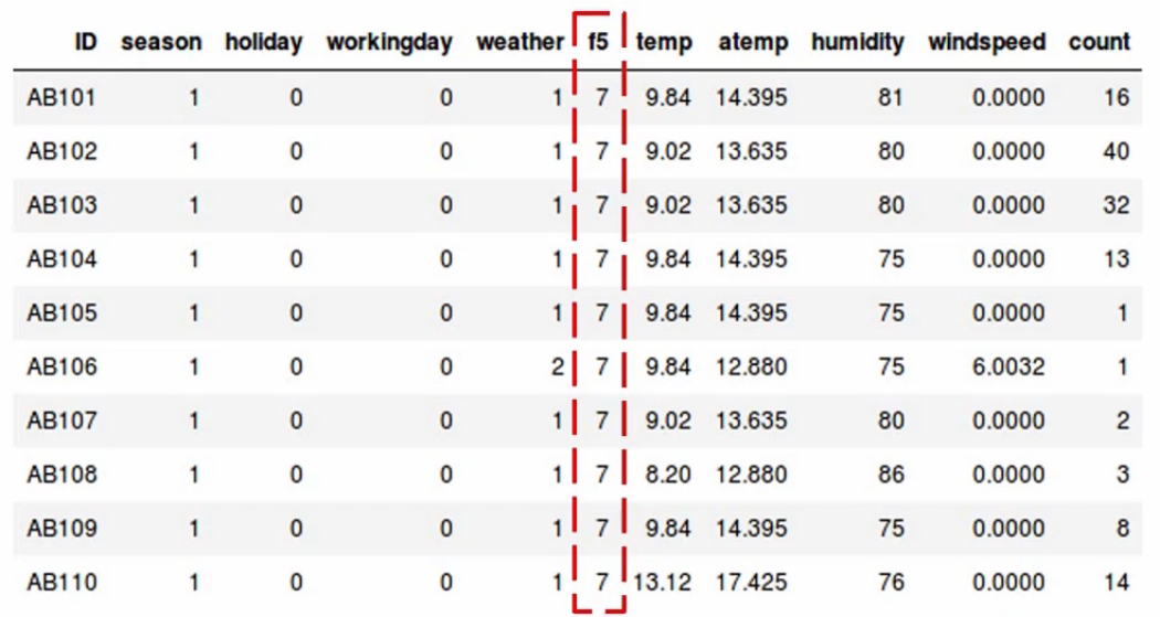
We have a constant value of 7 across all observations. Do you think the variable f5 will affect the value of count? Remember all the values of f5 are the same.
The answer is, No. It will not affect the count variable. If we check the variance of f5, it will come out to be zero.
Let me quickly recap what Variance is? and we’ll come back to this again.
Variance tells us about the spread of the data. It tells us how far the points are from the mean.
and the formula to calculate variance is given here-
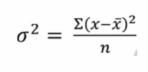
When we calculate the variance of the f5 variable using this formula, it comes out to be zero because all the values are the same. We can see that variables with low virions have less impact on the target variable. Next, we can set a threshold value of variance. And if the variance of a variable is less than that threshold, we can see if drop that variable, but there is one thing to remember and it’s very important, Variance is range-dependent, therefore we need to do normalization before applying this technique.
Implementation of Low Variance Filter
Not let’s implement it in Python and see how it works in a practical scenario. As always we’ll first import the required libraries-
#importing the libraries

import pandas as pd
from sklearn.preprocessing import normalize
We discuss the use of normalization while calculating variance. Hence, we are importing it into our implementation here. Don’t worry we’ll see where to apply it. Next, read the dataset-
#reading the file

data = pd.read_csv('low_variance_filter-200306-194411.csv')
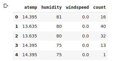
And let’s say, we’ll look at the first five observations-
# first 5 rows of the data

data.head()
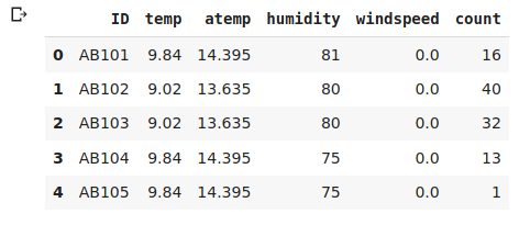
Again, have a few independent variables and a target variable, which is essentially the count of bikes. A quick look at the shape of the data-
#shape of the data

data.shape
It confirms we are working with 6 variables or columns and have 12,980 observations or rows. Now, let’s check whether we have missing values or not-
#percentage of missing values in each variable

data.isnull().sum()/len(data)*100
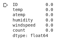
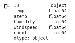
We don’t have any missing values in a data set. That’s great. Let me quickly see the data type or the variables. Why are we doing this? Remember we should apply the variance filter only on numerical variables. If we have categorical variables, we can look at the frequency distribution of the categories. And if a single category is repeating more frequently, let’s say by 95% or more, you can then drop that variable. But in our example, we only have numerical variables as you can see here-
#data type of variables

data.dtypes
So we will apply the low variance filter and try to reduce the dimensionality of the data. Before we proceed though, and go ahead, first drop the ID variable since it contains unique values for each observation and it’s not really relevant for analysis here-
#creating dummy variables of categorical variables

data = data.drop('ID', axis=1)
Let me just verify that we have indeed dropped the ID variable-
#shape of data

data.shape
and yes, we are left with five columns. Perfect! Our next step is to normalize the variables because variance remember is range dependent. And as we saw in our dataset, the variables have a pretty high range, which will skew our results. So go ahead and do that-
normalize = normalize(data)
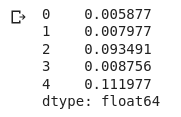
Save the result in a data frame called data_scaled, and then use the .var() function to calculate the variance-
data_scaled = pd.DataFrame(normalize)
data_scaled.var()
We’ll store the variance results in a new column and the column names in a different variable-
#storing the variance and name of variables

variance = data_scaled.var()
columns = data.columns
Next comes the for loop again. We’ll set a threshold of 0.006. So if the variable has a variance greater than a threshold, we will select it and drop the rest. So let me go ahead and implement that-
#saving the names of variables having variance more than a threshold value

variable = [ ]

for i in range(0,len(variance)):
    if variance[i]>=0.006: #setting the threshold as 1%
        variable.append(columns[i])
All right. So let’s see what we have-
variable
The temp variable has been dropped. The rest have been selected based on our threshold value. You can cross check it, the temp variable has a variance of 0.005 and our threshold was 0.006. That’s why it has been dropped here. Let’s move on and save the results in a new data frame and check out the first five observations-
# creating a new dataframe using the above variables
new_data = data[variable]

# first five rows of the new data
new_data.head()
Alright, it’s gone according to the plan. Now, code the variance of our remaining variables-
#variance of variables in new data
new_data.var()
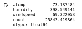
Do you notice something different? Yeah, that’s right. The variance is large because there isn’t any normalization here. Finally, verify the shape of the new and original data-
# shape of new and original data
new_data.shape, data.shape
Pretty much confirmed what we have done in this feature selection method to reduce the dimensionality of our data.
End Notes
In this article, we saw another common feature selection technique- Low Variance Filter. We also saw how it is implemented using python.
If you are looking to kick start your Data Science Journey and want every topic under one roof, your search stops here. Check out Analytics Vidhya’s Certified AI & ML BlackBelt Plus Program
If you have any queries let me know in the comments below!
I am a data lover and I love to extract and understand the hidden patterns in the data. I want to learn and grow in the field of Machine Learning and Data Science.


