A Step-By-Step Guide to AutoML with H2O Flow

Introduction

Isn’t it tiring to write multiple lines of code every time we wish to create a machine learning model!

Ever wondered how easy and efficient it would become if we could build a machine learning model by just pointing and clicking? H2O Flow provides a solution for all such problems!

H2O is an open-source machine learning and AI platform. It supports a web-based interface called Flow. H2O Flow can be used to create various types of machine learning models without writing any code. We can simply point and click to build machine learning pipelines. It has API support for R, Python, Scala.

In this article, we create models in H2O Flow by using AutoML but one might ask what exactly is AutoML and what’s the buzz about it?

Well to answer that, AutoML (Automated machine learning) simply automates the modeling process, which allows data scientists to focus on other crucial aspects of machine learning pipelines such as feature engineering and model deployment.

Learning Objectives

• Getting to know H2O Flow
  • H2O Installation
  • Running Flow web UI

• Data Loading
  • Importing data from the file system
  • Parsing the data

• Splitting into training and test data
• Run H2O AutoML
  • Introduction building models via AutoML
  • Model Exploration

• Analyze the leaderboard
  • Select the best model

• Prediction

Installing h2O Flow

Download the latest version of the software from the official page. You need to have64 bit java pre-installed as it is a prerequisite for H2O Flow. After the download is complete we can use the zip file with the H2O jar file.

Start the terminal, extract the file and follow the below commands to launch H2O Flow on your browser.

cd ~/Downloads

unzip h2o-3.30.0.6.zip
cd h2o-3.30.0.6
java -jar h2o.jar

Switch to your browser and navigate to http://localhost:54321 to gain access to the Flow web UI.

The first thing that might strike your mind would be the way Flow is designed is quite similar to Jupyter notebooks. The right panel is the help section and which can be insightful for beginners.

Do have a look at these keyboard shortcuts that will be used throughout the project!

Data Loading

We would be using the freely available dataset for our project. This data deals with direct marketing campaigns of a bank and we need to predict
the enrolment of their clients. based on many features. Study the dataset to know more about the features.

Now Let’s get started by creating our very own Flow notebook. Notice the “+” button at the top toolbar. We can use it to insert cells. Just like Jupyter notebooks, we can include markdown cells for any text we wish to write.

Click on the Import Files option and specify the location of the data file and start importing. We can also import files from other sources such as HDFS and S3 bucket.

Data Parsing

Data parsing refers to defining the schema. The schema is automatically detected for us by parse guesser. We can change any column as we like according to our needs. We can change the data type of categorical to enum, here we can change the ‘day’ column to enum as there are only 7 days in a week.

We know that this is a binary classification problem as we have to predict whether clients will enroll in term deposits or not.

Usually, we apply one-hot encoding on the categorical data before building a machine learning model but Flow provides us with an automatic one hot encoding feature. Now let’s go ahead and click Parse!

After the parsing is complete we can view the refined data including the size, columns, and rows.

Data Exploration

Let’s explore and visualize our data for better understanding. We can select the columns for visualizing them individually. We can get distribution for a numeric column or frequency count for categorical columns.

We can see the characteristics and summary of the “Age” column along with the frequency distribution.

Here, we can see the distribution for the “y” column. By visualizing the predictor column we conclude that there is a high level of class imbalance.

Similarly, we can check for other columns as well.

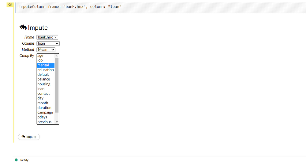
Flow has a provision for imputing the data. This can be useful in the case of a linear model that will impute through missing values. A number of methods are provided for imputation. The default method is set as Mean.

Creating Train and Test splits

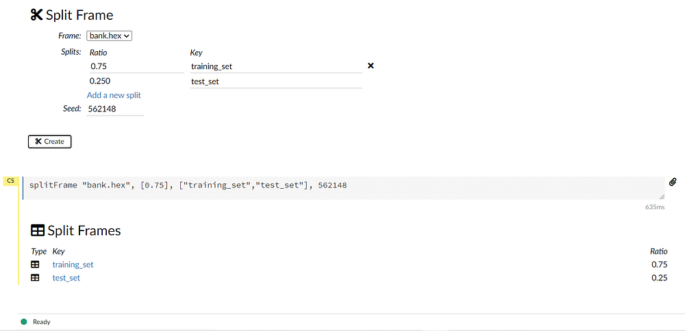
Before we start training our model we need to split our data into training and test sets. We can achieve this by navigating to data -> split frame from the toolbar.

Notice the default split is 75:25 for training and testing respectively. This can be modified according to needs. Rename the splits as “training_set” and “test_set”.

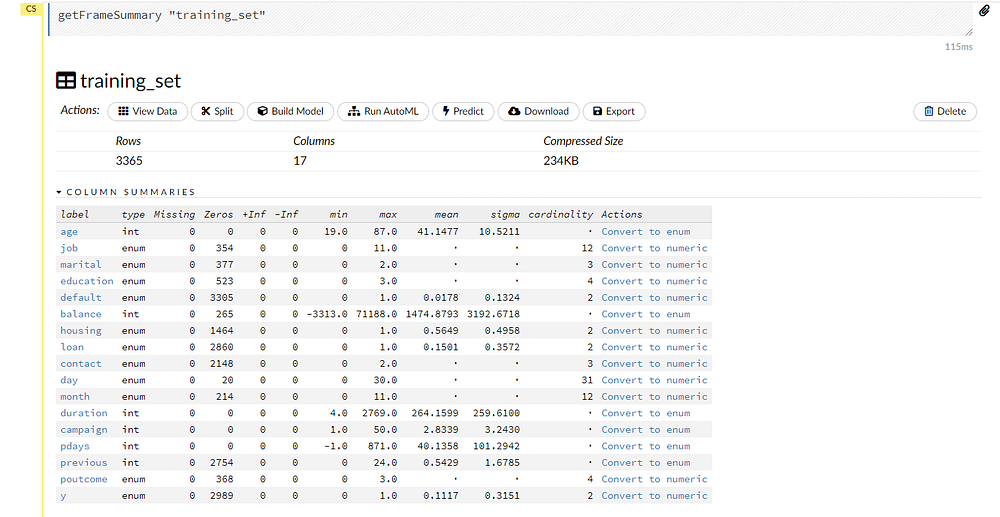
Now we can inspect each set individually by selecting the frames.

Building Model by AutoML

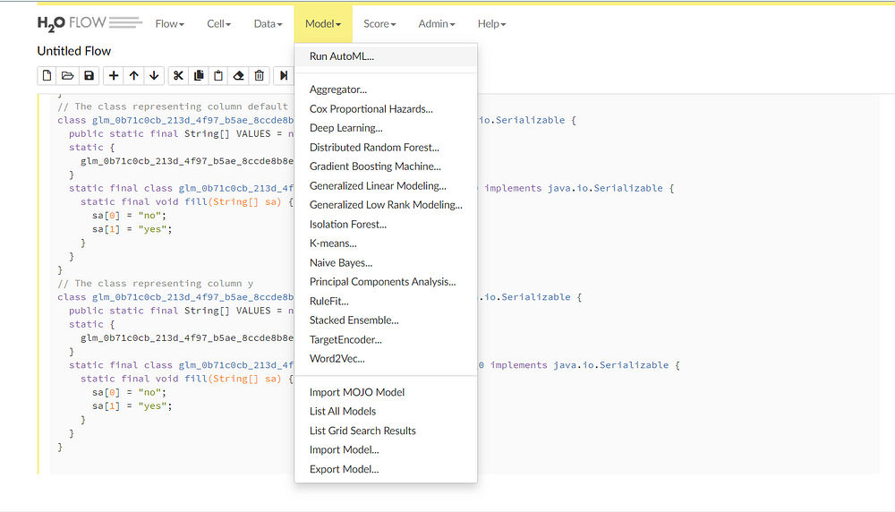
AutoML trains various types of models, including GLM’s random forests, distributed random forests, extreme random forests, deep learning XG boost, and stacked ensembles. It also presents a leaderboard with all the models sorted by some metrics.

We can select the Run AutoML option from the drop-down menu:

Now we can select the training frame, response frame and the validation frame as “training_set”, “y” and “test_set” respectively. We can ignore the other options as they are used to add advanced functionalities.

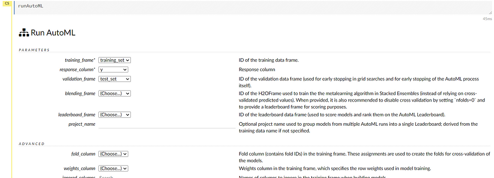
The cross-validation number is five by default. As we have a class imbalance situation we can select the balance classes option.

We can also exclude certain models if we know that they are not relevant. Change the max_runtime_seconds to 300 seconds.AutoML trains the models till the max_runtime_seconds after that it will stop. It is set to 3600 seconds by default.

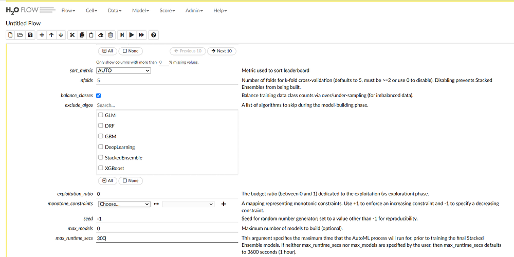
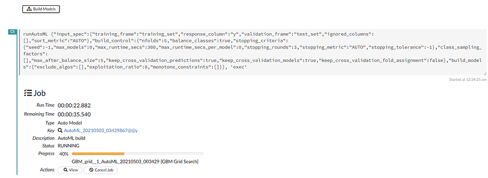
Finally, we can start building the models by selecting the “build models” option. There is an option for viewing the real-time updates of the models while training. We can also see the scoring history in real-time with graph representations.

Model Exploration

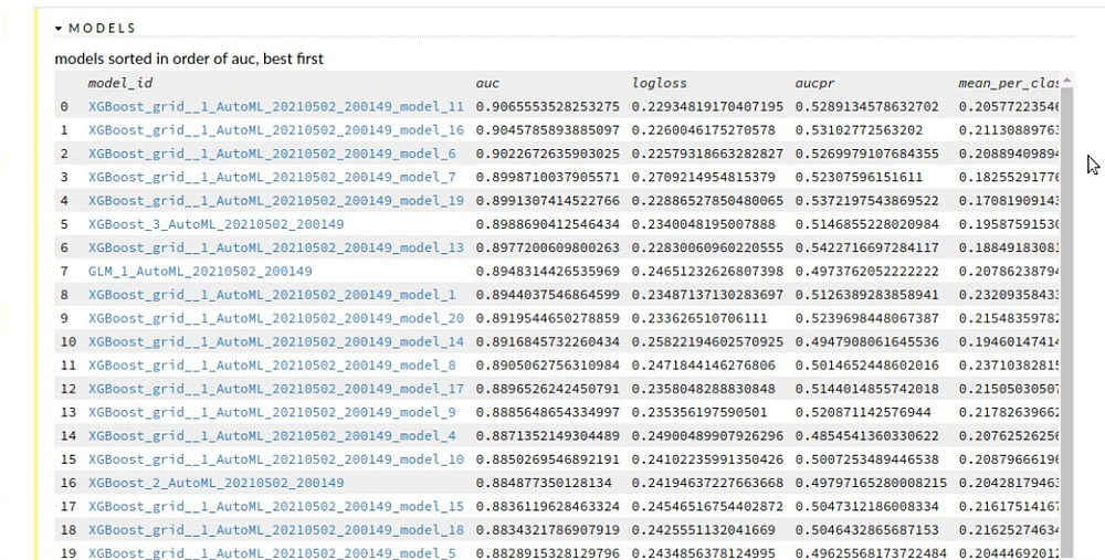
The training process will take five minutes as we specified max_runtime_seconds. After the job is completed we can navigate to the model leaderboard.

All the models trained by AutoML are displayed in a sorted order according to performance.

In this case, XGboost model is the best performing model.

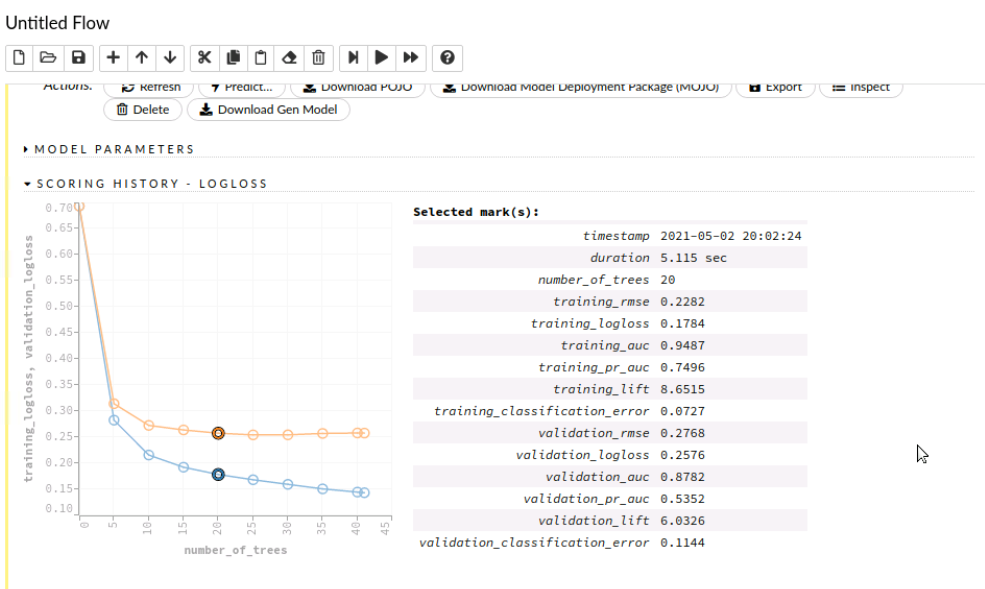
AutoML provides visualization of various metrics which can be used for model exploration. We can click on the curve to know more details about it.

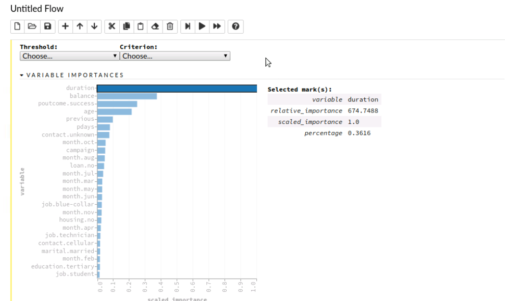
We can also check variable importance. We can see that the duration variable is highly predictive and is used by this model.

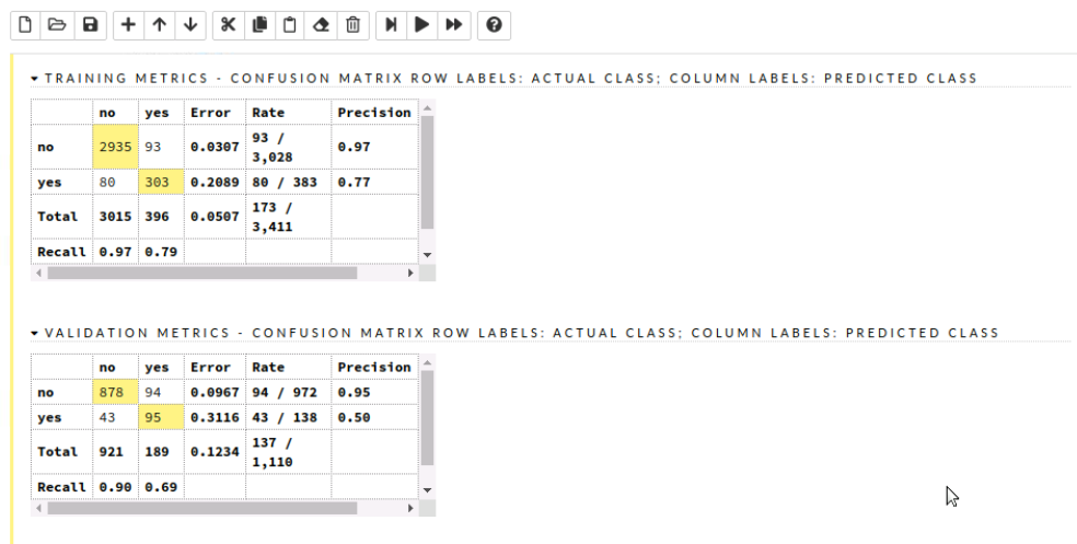
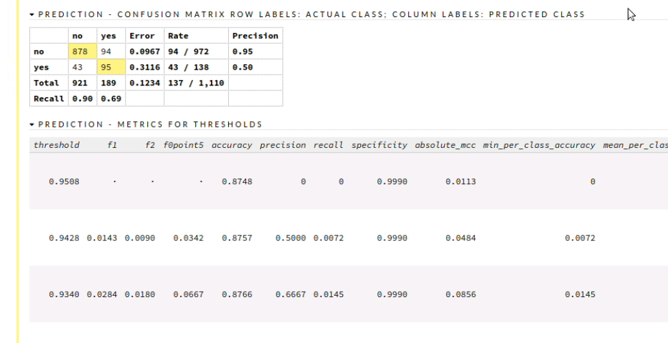
The confusion matrix is also crucial as they provide various insights such as correlation. We can also highlight particular variables and view them.

Prediction

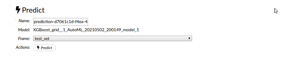
After we are satisfied with the selected model we can head over to making predictions.

Start by selecting predict option from the toolbar and select the model you want to use followed by selecting the validation frame. Now by simply clicking the predict button, we can view the predicted values along with various evaluation metrics such as the mean square.

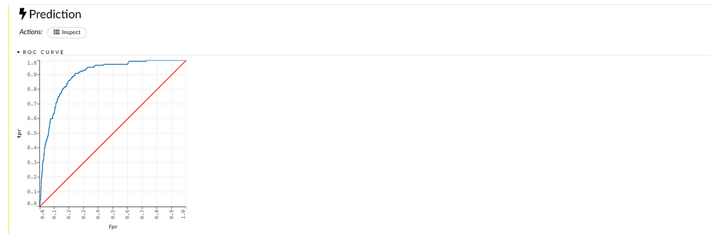
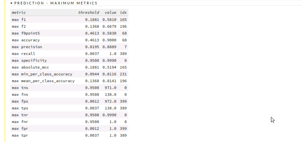
We can see the confusion matrix and analyze our result along with various metrics and graph representations.

End Notes

We have successfully learned to use H20 from the Web-based UI called H2O Flow and have trained and visualized models without writing a single line of code!! Through this article, you might have an idea of how easy machine learning modeling becomes with the use of AutoML. I highly encourage you to study the official documentation for more information.