Boruta with R is a great way to address the “Curse of Dimensionality”.

This article was published as a part of the Data Science Blogathon.

Introduction

Machine Learning is based on the idea that you receive back exactly what you put in. You will only receive trash if you offer trash. The term “trash” here refers to the noise. This is a common misunderstanding that the more features we have in our learning model, the more accurate it would be. However, this is not the scenario; not all of the features are equally important and will aid our model’s accuracy.

The number of features and model performance does not have a linear relationship, as seen in the following diagram. The model’s accuracy increases up to a certain threshold value, but after that, if we add more dimensions, the model’s accuracy will only get worse. The “Curse of Dimensionality” is the name given to this problem.

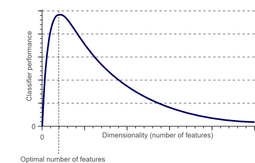
The drawbacks of adding unnecessary dimensions to data.

1.  It will be time-consuming. The model will take more time to get trained on the data.
2. The accuracy of the model may also be impacted.
3. The model is prone to a problem known as “Overfitting”.

Assume the two dimensions/features are strongly correlated, and that one can be found using the other one. In this case, iterating over the second feature would simply consume more time without adding improvement to the model’s accuracy.

This becomes one of the most challenging problems to deal with whenever we have a lot of features in our data. We use a technique known as “Feature Selection” to address this issue. Only the most significant features are chosen in this technique. As a consequence, accuracy may also get improved and lesser time will be consumed

Methods for Feature Selection

Src: https://images.app.goo.gl/Nv4YTfb2oXsjCbmw5

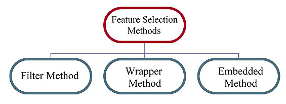
1) Filter Method

This approach takes all of the subsets of features and, after picking them all, attempts to determine the optimal subset of features using various statistical methods. Correlation Coefficient (Pearson, Spearman), ANOVA test, and Chi-Square test are examples of statistical techniques used.

All features that have a strong relationship with the target variable are picked. After picking the optimal subset, the machine learning algorithm is trained on it and its accuracy is evaluated.

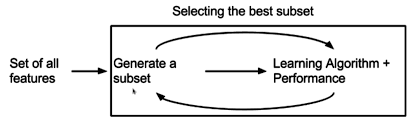
2) Wrapper Method

It’s easier than the filter approach because statistical tests aren’t required. Wrapper methods are classified as follows:

Forward Selection: The method starts with no characteristics. Later continues to add characteristics to the model that increase its accuracy with each iteration.

Backward Selection: It starts with all the features and then eliminates those that increase the model’s accuracy in each iteration. The process will be repeated until no improvement in the elimination of any feature is detected.

Recursive Feature Elimination: This technique employs the greedy strategy. It doesn’t have all of the features. It tries to identify the most significant features. It will only accept them.

3) Embedded Method

This approach creates various subsets of features in all feasible combinations and permutations. It then chooses the subset that will provide the best accuracy.

Src: https://images.app.goo.gl/xTqxNRvnbjuGF56V8

We will learn about the ‘Boruta’ algorithm for feature selection in this article. Boruta is a Wrapper method of feature selection. It is built around the random forest algorithm. Boruta algorithm is named after a monster from Slavic folklore who resided in pine trees. 

Src: https://images.app.goo.gl/RPwe1n1RnfHSMZWM9

But, exactly, how does this algorithm work? Let’s explore…

Working of Boruta

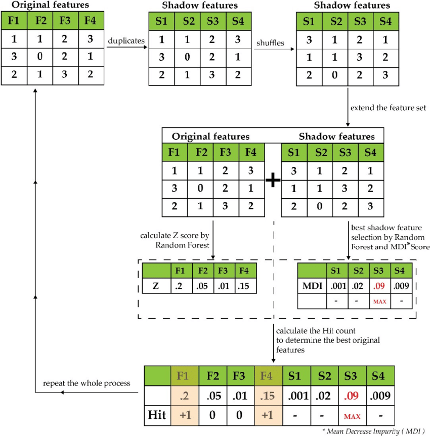
• The independent variables’ shadow features are generated by Boruta. Shadow features are duplicates of the original independent features with adequate shuffling, as seen in the Figure below. This shuffle is performed to eliminate the correlation between the independent and the target attribute. Here S1, S2, and S3 are the shadow features of the original features F1, F2, and F3.

Src: https://images.app.goo.gl/3WczMzeyc5uQjYzH7

• The algorithm would then merge both the original and shadow features in the second step.
• Pass this combined data to the random forest algorithm. This provides the importance of the features via Mean Decrease Accuracy/Mean Decrease Impurity.
• Random Forest determines the Z score for both original and shadow features based on this. Compare the shadow features’ maximum Z score to the individual original features’ Z score.
• The algorithm uses the shadow features’ maximum Z score as the threshold value. The original features with a Z score higher than the max shadow feature are deemed “significant,” while those with a Z score lower than that are deemed “unimportant”.
• This procedure is repeated until all the important and unimportant features have been identified, or other termination conditions have been met.

 

Using R to implement Boruta

• Step 1:

Load the following libraries:

library(caTools)
library(Boruta)
library(mlbench)
library(caret)
library(randomForest)

• Step 2:

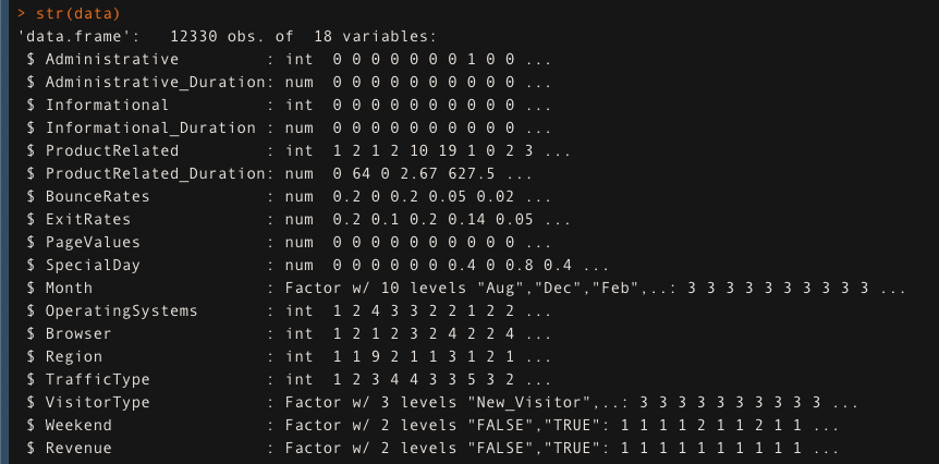
we will use online customer data in this example. It contains 12330 observations and 18 variables. Here the str() function is used to see the structure of the data

data <- read.csv(onlineshopping.csv, header =T)
str(data)

• Step 3:

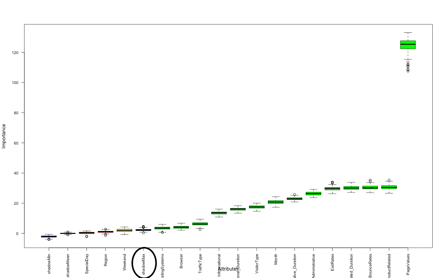
Now we will use the ‘Boruta’ function to find the important and unimportant attributes. All the original features having a lesser Z score than shadow max (circled in the plot below) will be marked unimportant and after this as important.

set.seed(123)
boruta_res <- Boruta(Revenue~., data= data, doTrace=2, maxRuns= 150)
plot(boruta_res, las=2, cex.axis=0.8)

• Step 4:

Split the data into ‘train’ & ‘test’. 75% for training and the rest 25% for testing.

set.seed(0)
split <- sample.split(data,SplitRatio = 0.75)
train <- subset(data,split==T)
test <- subset(data,split==F)

• Step 5:

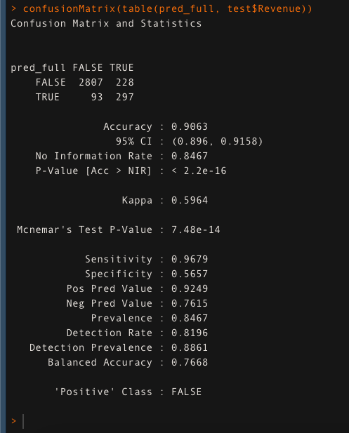
Check the accuracy of the random forest model when all the features are used to train the model. Here all 17 independent features are used. It is providing an accuracy of 90.63%

rfmodel <- randomForest(Revenue ~., data = train)
pred_full <- predict(rfmodel, test)
confusionMatrix(table(pred_full, test$Revenue))

• Step 6:

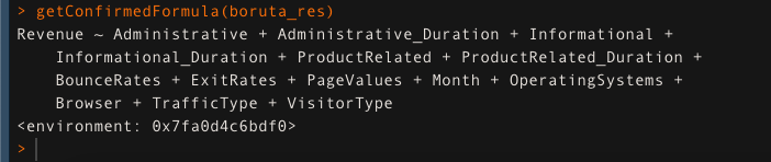
Get the formula for all the important features using the ‘getConfirmedFormula()’ function. Here 14 features are confirmed as important.

getConfirmedFormula(boruta_res)

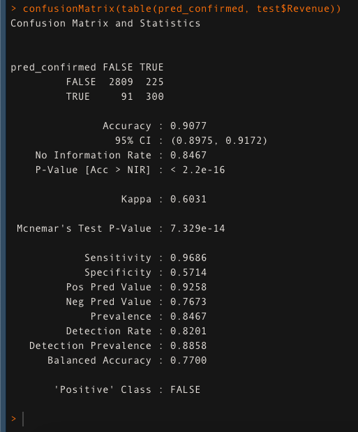
• Step 7:

Checking the accuracy of the model when trained with only important attributes. In this case, the model is giving an accuracy of 90.77% which is slightly more than the previous model even though only 14 out of 17 attributes are used.

rfmodel <- randomForest(Revenue ~ Administrative + Administrative_Duration + Informational +
                       Informational_Duration + ProductRelated + ProductRelated_Duration +
                       BounceRates + ExitRates + PageValues + Month + OperatingSystems +
                       Browser + TrafficType + VisitorType, data = train)
pred_confirmed <- predict(rfmodel, test)
confusionMatrix(table(pred_confirmed, test$Revenue))

Article by~

Shivam Sharma & Dr Hemant Kumar Soni.

Shivam Sharma 01 Jul 2021