Gradient Descent From Scratch

This article was published as a part of the Data Science Blogathon

Gradient Descent is one of those topics which sometimes scare beginners and practitioners. I have seen most people when heard the term Gradient then they try to finish the topic without understanding Maths behind it. In this tutorial, I will explain your Gradient descent from a very ground level, And pick you up with simple maths examples, and make gradient descent completely consumable for you.

Table of Contents

• What is Gradient Descent and why it is important?
• Intuition Behind Gradient Descent
• Mathematical Formulation
• Code for Gradient Descent with 1 variable
• Gradient Descent with 2 variable
• Effect of Learning Rate
• Effect of Loss Function
• Effect of Data
• EndNote

What is Gradient Descent?

Gradient Descent is a first-order optimization technique used to find the local minimum or optimize the loss function. It is also known as the parameter optimization technique.

Why Gradient Descent?

It is easy to find the value of slope and intercept using a closed-form solution But when you work in Multidimensional data then the technique is so costly and takes a lot of time Thus it fails here. So, the new technique came as Gradient Descent which finds the minimum very fastly.

Gradient descent is not only up to linear regression but it is an algorithm that can be applied on any machine learning part including linear regression, logistic regression, and it is the complete backbone of deep learning.

The intuition behind Gradient Descent

considers I have a dataset of students containing CGPA and salary package.

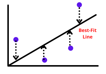
We have to find the best fit line that gives a minimum value of b when the loss is minimum. The loss function is defined as the squared sum of the difference between actual and predicted values.

To make the problem simple to understand Gradient descent suppose the value of m is given to us and we have to predict the value of intercept(b). so we want to find out the minimum value of b where L(loss) should be the minimum.

So, if we plot the graph between L and b then it will be a parabolic shape. Now in this parabola, we have to find the minimum value of b where loss is minimum. want  If we use ordinary least squares, it will differentiate and equate it to zero. But this is not convenient working with high-dimensional data. So, here comes Gradient Descent. let’s get started with performing Gradient Descent.

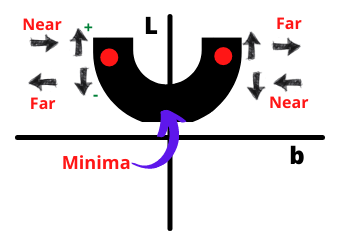
Select a random value of b

we select any random value of b and find its corresponding L value. Now we want to converge it to the minimum.

On the left side, if we increase b then we are going towards minimum and if decreasing then we are going away from the minimum. On the right side, if we decrease b then we are going closer to a minimum and on increasing we are going away from the minimum. Now how would I know that I want to go forward or backward?

So, The answer is simple, We find the slope at the current point where we stand. Now again the question may arise How to find a slope? To find the slope we differentiate the equation os loss function which is the equation of slope and on simplifying we get a slope.

Now the direction of the slope will indicate that you have to move forward or backward. If a slope is positive then we have to decrease b and vice-versa. in short, we subtract the slope from the old intercept to find a new intercept.

b_new = b_old - slope

This is only the equation of gradient and Gradient means derivative if you have more than one variable as slope and intercept. Now again question arise is that How would I know where to stop? we are going to perform this convergence step multiple times in a loop so it is necessary to know when to stop.

one more thing is, if we subtract the slope there is a drastic change in movement it is known as a zig-zag movement. To avoid this case we multiply the slope with a very small positive number known as the learning rate.

Now the equation is

      bnew = bold - learning rate * slope

hence, this is why we use the learning rate to reduce the drastic change in step size and direction of the movement. We will see the effect and use of the learning rate in deep further in this tutorial.

Now the question is the same when to stop the loop? so there are 2 approaches when we stop moving forward.

1. when b_new – b_old = 0 means we are not moving forward so we can stop.
2. we can limit the number of iterations by 1000 times. Several iterations are known as epochs and we can initialize it as Hyperparameter.

This is the Intuition behind the Gradient descent. we have only covered the theory part till And now we will start Mathematics behind Gradient descent and I am pretty sure you will get it easily.

Maths behind Gradient Descent

consider a dataset, we did not know the initial intercept. we want to predict the minimum value of b and for now, we are considering we know the value of m. we have to apply gradient descent to only know the value of b. the reason behind this is understanding with one variable will be easy and in this further article, we will implement the complete algorithm with b and m both.

step-1) start with a random b

At the start, we consider any random value of b and start iteration in for loop and find the new values for b with help of slope. now suppose the learning rate is 0.001 and epochs is 1000.

Step-2) Run the iterations

for i in epochs:
  b_new = b_old - learning_rate * slope

Now we want to calculate the slope at the current value of b. So we will calculate the equation of slope with help of the loss function by differentiating it concerning b.

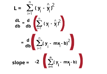
That’s simple it is calculating slope, and simply you can put the values and calculate the slope. The value of m is given to us so it is easier. And we will do this thing till all iterations get over.

This is only the Gradient Descent and you only need to this much. we have seen How gradient descent works and Now let’s make our hands dirty by implementing gradient descent practically using Python.

Making Hands dirty by Implementing Gradient Descent with 1 variable

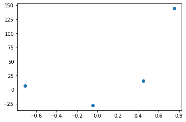
here, I have created a very small dataset with four points to implement Gradient descent on this. And the value of m we are given so we will first try the Ordinary least square method to get m and then we will implement Gradient descent on the dataset.

Get the value of m with OLS

from sklearn.linear_model import LinearRegression
reg = LinearRegression()
reg.fit(X,y)
print(reg.coef_)
print(reg.intercept_)

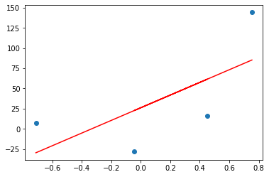
After applying OLS we get the coefficient, value of m as 78.35 and intercept as 26.15. Now we will implement Gradient descent by taking any random value of intercept and you will see that after performing 2 to 3 iteration we will reach near 26.15 and that is our end goal to implement.

If I plot the prediction line by OLS then it will look something like this.

plt.scatter(X,y)
plt.plot(X,reg.predict(X),color='red')

Now we will implement Gradient descent then you will see that our gradient descent predicted line will overlap it as iteration increases.

Iteration-1

Let’s apply Gradient descent assuming slope is constant at 78.35 and a starting value of intercept b is 0. so let us apply the equation and predict the initial value.

y_pred = ((78.35 * X) + 0).reshape(4)
plt.scatter(X,y)
plt.plot(X,reg.predict(X),color='red',label='OLS')
plt.plot(X,y_pred,color='#00a65a',label='b = 0')
plt.legend()
plt.show()

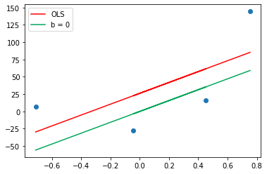
This is a line when an intercept is zero and Now as we will move forward by calculating the slope and find a new value of b will move towards the red line.

m = 78.35
b = 0
loss_slope = -2 * np.sum(y - m*X.ravel() - b) 
# Lets take learning rate = 0.1
lr = 0.1
step_size = loss_slope*lr
print(step_size)
# Calculating the new intercept
b = b - step_size
print(b)

When we calculate the learning rate multiplied by slope is known as step size and to calculate the new intercept we subtract step size from the old intercept and that’s what we have done. And the new intercept is 20.9 hence directly from 0 we have reached 20.9.

Iteration – 2

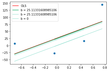
Now again we will calculate the slope at intercept 20 and you will see it will move very near to the required intercept of 26.15. The code is the same as above.

loss_slope = -2 * np.sum(y - m*X.ravel() - b)
step_size = loss_slope*lr
b = b - step_size
print(b)

Now the intercept is 25.1 which is very near to the required intercept. If you run one more iteration then I am sure you will get the required intercept and the green line will overtake the red one. And on plotting you can see the graph as below in which the green line overtakes the red.

 

From the above experiment, we can conclude that when we are far from minima we take long steps and as we reach near to minima we take small steps. This is the beauty of Gradient Descent that even when you start with any wrong point say 100, then also after some iteration, you will reach the correct point And this is all due to learning rate.

Gradient Descent for 2 Variables

Now we can understand the complete working and intuition of Gradient descent. Now we will perform Gradient Descent with both variables m and b and do not consider anyone as constant.

Step-1) Initialize the random value of m and b

here we initialize any random value like m is 1 and b is 0.

Step-2) Initialize the number of epochs and learning rate

take learning rate small as possible suppose 0.01 and epochs as 100

Step-3) Start calculating the slope and intercept in iterations 

Now we will apply a loop for several epochs and calculate slope and intercept.

for i in epochs:
  b_new = b_old - learning_rate * slope
  m_new = m_old - learning_rate * slope

The equation is the same as we have derived above by differentiation. here we have to differentiate the equation 2 times. one concerning b(intercept) and one concerning m. This is Gradient Descent.

Now we will build the Gradient Descent complete algorithm using Python for both variables.

Implement Complete Gradient Descent Algorithm with Python

from sklearn.datasets import make_regression
X, y = make_regression(n_samples=100, n_features=1, n_informative=1, n_targets=1, noise=20, random_state=13)

This is the dataset we have created, Now you are free to apply OLS and check coefficients and intercept. let us build a Gradient Descent class.

class GDRegressor:
  def __init__(self, learning_rate, epochs):
    self.m = 100
    self.b = -120
    self.lr = learning_rate
    self.epochs = epochs
  def fit(self, X, y):
    #calculate b and m using GD
    for i in range(self.epochs):
      loss_slope_b = -2 * np.sum(y - self.m * X.ravel() - self.b)
      loss_slope_m = -2 * np.sum((y - self.m * X.ravel() - self.b)*X.ravel())
      self.b = self.b - (self.lr * loss_slope_b)
      self.m = self.m - (self.lr * loss_slope_m)
    print(self.m, self.b)
  def predict(self, X):
    return self.m * X + self.b
#create object and check algorithm
gd = GDRegressor(0.001, 50)
gd.fit(X, y)

I am pursuing my Bachelor of Technology(B-Tech) in Information Technology. I am an enthusiast of learning and very much fond of data science and Machine learning. Please feel free to connect with me on Linkedin.

The media shown in this article are not owned by Analytics Vidhya and is used at the Author’s discretion.

Raghav Agrawal 30 Oct 2022

I am a final year undergraduate who loves to learn and write about technology. I am a passionate learner, and a data science enthusiast. I am learning and working in data science field from past 2 years, and aspire to grow as Big data architect.