GreyKite : Time Series Forecasting in Python

This article was published as a part of the Data Science Blogathon

Introduction

Time Series Forecasting is a very important problem in machine learning. It is important because time is there as a feature in these problems. There are a lot of different real-life examples you can see related to time series forecasting like predicting the sales of a store with respect to a number of days.

In this blog, we are going to read a new time series forecasting library in python GreyKite. This is released by LinkedIn and it helps to automate time series problems. So let’s get started.

Check my latest articles here

Image Source

Table of Contents

• GreyKite
• Features of GreyKite
• Problem Statement
• Installation
• Import Libraries
• Read Dataset
• Create a Forecast
• Cross-Validation
• Backtest
• Forecast
• Model Diagnostics

GreyKite

This brand new Python library GreyKite is released by Linkedin. It is used for time series forecasting. This library makes the life of data scientists easier. This library provides automation with the help of the Silverkite algorithm. LinkedIn created GrekKite to help its group settle on viable choices dependent on the time-series forecasting models. This also helps to interpret the outputs. If you want to know more about this library then check the official documentation here.

Image Source

Algorithms supported by Gryekite library

Throughout the long term, LinkedIn has been utilizing the Greykite library to give an adequate foundation to deal with top traffic, set business targets, and advance spending choices.

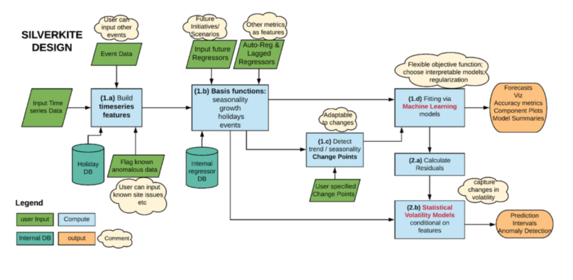
Image Source

Features of GreyKite

Fast training and scoring

Flexible design

Intuitive Interface

Extensible Framework

Image Source

Installation

For analysis, we need to install the GreyKite library. Check the below command to install the library. Type the below command in the command line prompt. For more information, check the below code.

%matplotlib inline
!pip install -qqq greykite

Import Libraries

In this section, we are going to import all the required libraries that are useful for further analysis. We will be using Pandas, collections, plotly, matplotlib, and Greykite. For more information, check the below code.

from collections import defaultdict
import warnings
import pandas as pd
warnings.filterwarnings("ignore")
import pandas as pd
import plotly
from greykite.framework.templates.autogen.forecast_config import ForecastConfig
from greykite.framework.templates.autogen.forecast_config import MetadataParam
from greykite.framework.templates.forecaster import Forecaster 
from greykite.framework.templates.model_templates import ModelTemplateEnum
from greykite.framework.utils.result_summary import summarize_grid_search_results

Read Dataset

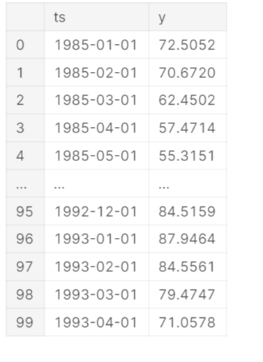
In this section, we are going to read data. We are using Pandas read_csv() function. I am changing the data type of the DATE parameter using astype() function. After this, rename the column DATE as ts and Value as y. We are using the head() function and passing the parameter 100 to show the first 100 rows of the dataset. Check the below code for more information.

df = pd.read_csv('electric-production/Electric_Production.csv')
df['DATE'] = df['DATE'].astype('datetime64[ns]')
df.rename(columns = {'DATE': 'ts', 'Value': 'y'}, inplace = True)
df = df.head(100)
df

Create a Forecast

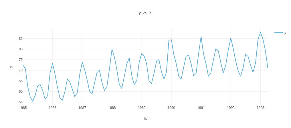
The forecast can be created with just a few lines of code. First, specify the dataset information. We are setting the time_col parameter as ts and the value_col parameter as y. In freq, we are setting value as MS for Monthly at the start date. After this create a forecaster using the Forecaster class from the GreyKite package. The output of run_forecast_config() would be a dictionary which is having future predicted values, original time series, and historical forecast performance. Check the below code for complete information.

# Specifies dataset information
metadata = MetadataParam(
     time_col="ts",  # name of the time column
     value_col="y",  # name of the value column
     freq="MS"  #"MS" for Montly at start date, "H" for hourly, "D" for daily, "W" for weekly, etc.
 )
forecaster = Forecaster()
result = forecaster.run_forecast_config(
     df=df,
     config=ForecastConfig(
         model_template=ModelTemplateEnum.SILVERKITE.name,
         forecast_horizon=100,  # forecasts 100 steps ahead
         coverage=0.95,  # 95% prediction intervals
         metadata_param=metadata
    )
)

ts = result.timeseries
fig = ts.plot()
plotly.io.show(fig)

Cross-Validation

As a matter of course, run_forecast_config gives chronicled assessment, so you can perceive how the conjecture performs on past information. This is put away in grid_search (cross-approval parts) and backtest (holdout test set).

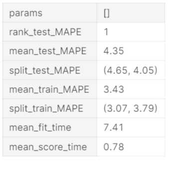
How about we check the cross-validation results. Naturally, all measurements in Element-wise Evaluation Metric Enum are registered on every CV train/test split. The setup of CV assessment measurements can be found at Evaluation Metric. Underneath, we show the Mean Absolute Percentage Error (MAPE) across parts

grid_search = result.grid_search
 cv_results = summarize_grid_search_results(
     grid_search=grid_search,
     decimals=2,
     # The below saves space in the printed output. Remove to show all available metrics and columns.
     cv_report_metrics=None,
     column_order=["rank", "mean_test", "split_test", "mean_train", "split_train", "mean_fit_time", "mean_score_time", "params"])
 # Transposes to save space in the printed output
 cv_results["params"] = cv_results["params"].astype(str)
 cv_results.set_index("params", drop=True, inplace=True)
 cv_results.transpose()

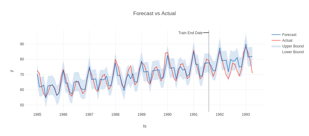
Backtest

Let’s plot the historical forecast on the holdout test set. Check the below code for more information.

backtest = result.backtest
fig = backtest.plot()
plotly.io.show(fig)

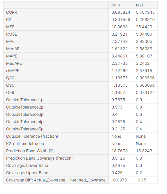
Check the historical evaluation metrics(on the historical test/train set) using the below code

backtest_eval = defaultdict(list)
 for metric, value in backtest.train_evaluation.items():
     backtest_eval[metric].append(value)
     backtest_eval[metric].append(backtest.test_evaluation[metric])
 metrics = pd.DataFrame(backtest_eval, index=["train", "test"]).T
 metrics

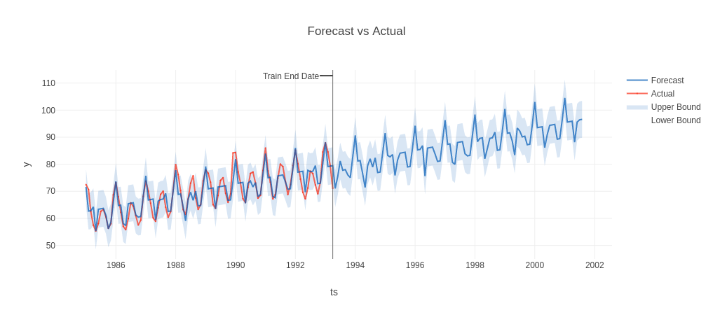
Forecast

In this section, we are going to plot the forecasted values. The forecast attribute having a forecasted value. Let’s plot the forecasted values using the below code. For more information, check the below code.

forecast = result.forecast
fig = forecast.plot()
plotly.io.show(fig)

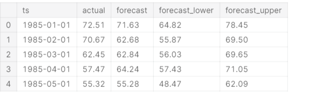
You can also check the forecasted values using the head() function. All the forecasted values are there in df. For more information, check the below code.

forecast.df.head().round(2)

Model Diagnostics

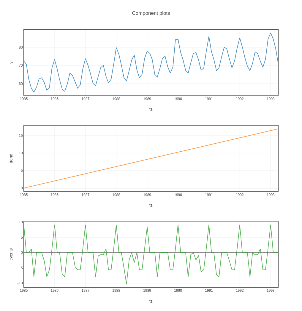
In this section, we are going to see model diagnostics. There are one more plot function plot_components(), this plot shows how your dataset’s trend, event/holiday, seasonality patterns are handled in the model. For more information, check the below code.

fig = forecast.plot_components()
plotly.io.show(fig)     # fig.show() if you are using "PROPHET" template

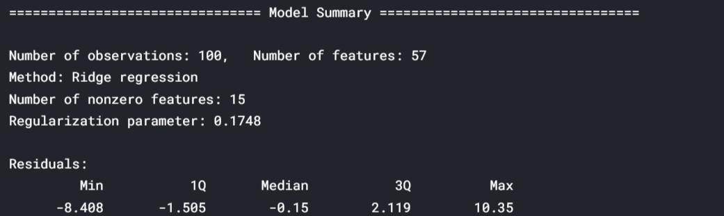
The model summary allows inspection of individual model terms. Check parameter estimates and their significance for insights on how the model works and what can be further improved.

summary = result.model[-1].summary()  # -1 retrieves the estimator from the pipeline
 print(summary)

End Notes

So in this article, we had a detailed discussion on Time Series Forecasting Using GreyKite Python Library. Hope you learn something from this blog and it will help you in the future. Thanks for reading and your patience. Good luck!

You can check my articles here: Articles

Email id: [email protected]

Connect with me on LinkedIn: LinkedIn.

The media shown in this article are not owned by Analytics Vidhya and are used at the Author’s discretion.

Akshay Gupta 31 May 2021