Image Raster Analysis: Spatial Correlation

This article was published as a part of the Data Science Blogathon.

Correlation Test

Assessing the relationship between two variables is commonly performed in science or experiment. A correlation test is performed to get the correlation coefficient and p-value. The correlation coefficient tells how strong the relationship is and the p-value tells whether the correlation test is significant. Then, we can conclude if a dependent variable affects a target variable.

This is a common method to use in analyzing tabular data. This article will also discuss how to do a correlation test, but for spatial data, especially raster data. The raster data is the image with spatial attributes. Performing a correlation test to spatial raster is similar to that for tabular data.

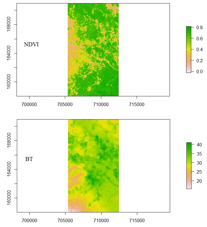
Let say, we have two sets of raster data: (1) NDVI (Normalized Difference Vegetation Index) and (2) Brightness Temperature (BT). Then, we want to test the relationship between the two to know whether vegetation affects temperature. NDVI represents vegetation condition. NDVI above 0.6 is usually high-density vegetation, like a forest. NDVI from 0.4 to 0.6 is usually crop. NDVI from 0.2 to 0.4 is usually soil, bare land, or houses. NDVI with a negative number is usually water body.

The first thing to do is overlaying both the raster datasets together. Next, convert them from raster into tabular. Each of the pairing cells or pixels will be arranged side by side in the table. So, the table has 2 columns for NDVI and BT. The table has the number of rows as much as the cell number. After that, we can just run the correlation test.

But, we do not always get raster datasets with the same resolution or cell size, and coverage area. In this example, NDVI is processed using Band 5 and Band 4 of Landsat 8 OLI with a cell size of 30 meters. Brightness Temperature has a cell size of 90 meters. Both raster datasets have different cell sizes and also different coverage areas. After they are overlaid together, they cannot be converted into a data frame because the cells do not pair with each other. Figure 1 illustrates 2 sets of raster images. The black raster has a higher resolution than the red raster does. The cells do not match.

Resampling Cell Size

Here is the challenge for spatial analysis. Before running the correlation test, we must process both the raster images to have the same cell size and coverage area. Every cell of the NDVI raster must coincide with every cell of the BT raster respectively. To do this, before overlaying the raster images, we need to resample one of the raster data according to another raster cell size. The option now is whether to resample NDVI raster according to BT raster or vice versa.

If the NDVI raster is resampled according to the BT raster, then the 30-meter cell size is generalized to 90 meters. There will be some missing information in it. If BT raster with the 90-meter resolution is resampled into 30-meter resolution, there will synthetic information from the interpolation. In spatial data, it is more preferable to generalize complicated data into simpler data than vice versa. So in this case, we are going to resample the NDVI raster so that the cell resolution is 90 meters.

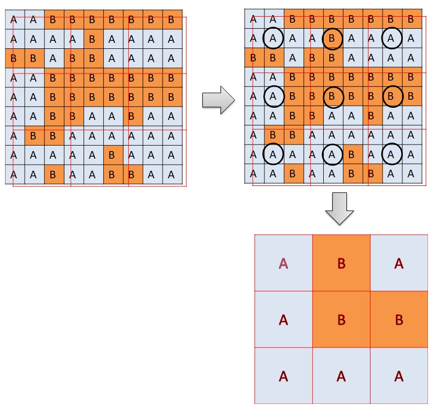
There are two methods of resampling in “raster” package. The first method “ngb” is used to resample categorical values according to the “nearest-neighbor”. Another method is “bilinear” used for resampling continuous values by interpolation. In this case, bilinear interpolation is used

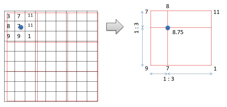
The method “ngb” creates a new raster with the cell values according to the nearest values of the old raster. Bilinear interpolation creates a new raster with the cell values based on the 4 nearest values of the old raster. Please observe Figure 3. A new cell is created. The value of the new raster is on the blue dot. There are four cells surrounding the blue dots. They are 7, 9, 1, and 11. The value of the blue dot is the weighted average of the 4 surrounding values according to the distance.

Below is the code for importing the needed packages, loading datasets, and resampling the NDVI raster.

# Import packages
library(raster)
library(tidyverse)
# Load data
bt <- raster(file.path("D:/bt_c.tif"))
ndvi <- raster(file.path("D:/ndvi_c.tif"))
# Resample the ndvi based on bt
ndvi <- resample(ndvi, bt, method="bilinear")

Masking Raster

After resampling the NDVI image, now we can convert the two images into a data frame with pairing cells. The next challenge is to solve no-value cells. There are areas with NDVI values, but no BT values. There are also areas with BT values, but no NDVI values. We do not want these areas to be included in the correlation test. Usually, areas with no values are filled with outstanding numbers, such as 0, 9999, or -9999. This will ruin the correlation test.

To filter out those areas, we need to mask both the raster datasets with each other. It means that the cells with no value for either NDVI or BT are removed. It is the same as the intersection. Only cells with available values from both raster datasets are returned. Below is the code to perform raster masking.

# Masking rasters
ndvi_m <- mask(ndvi, bt)
bt_m <- mask(bt, ndvi)
# Plot
plot(ndvi_m)
plot(bt_m)

Converting to Data Frame and Running Correlation Test

Now that resampling and masking have been done, both the raster datasets can be converted into a data frame. As mentioned earlier, the data frame has a column for NDVI values and another column for BT values. Each row is the pairing cell. A correlation test now can be performed to test the relationship. In this case, Pearson correlation is used as both of the variables are continuous. Below is the code to get the correlation coefficient and p-value.

# Overlay 2 rasters and create the data frame
overlay <- stack(ndvi_m, bt_m)
overlay <- data.frame(na.omit(values(overlay)))
names(overlay2) <- c("ndvi", "bt")
# correlation test
cor.test(overlay[,1], overlay[,2])

Output:

Pearson's product-moment correlation
data:  overlay[, 1] and overlay[, 2]
t = 6.1095, df = 31557, p-value = 1.011e-09
alternative hypothesis: true correlation is not equal to 0
95 percent confidence interval:
 0.02334775 0.04538748
sample estimates:
      cor 
0.0343718

Here are the first 7 rows of the data look.

We can see that the correlation coefficient is 0.0343718 and the p-value is 1.011e-09. It means that NDVI does not affect Brightness Temperature.

We can also perform other kinds of analysis. For example, let’s perform linear regression with NDVI as the independent variable and BT as the target variable. Below is the code.

# linear regression (alternative)
linear <- lm(overlay[,1] ~ overlay[,2])
summary(linear)

Output:

Call:
  lm(formula = overlay[, 1] ~ overlay[, 2])
Residuals:
  Min       1Q   Median       3Q      Max 
-0.48114 -0.14726  0.01716  0.16513  0.28196
Coefficients:
             Estimate Std. Error t value Pr(>|t|)    
(Intercept)  0.4453772  0.0091248   48.81  < 2e-16 ***
  overlay[, 2] 0.0017075  0.0002795    6.11 1.01e-09 ***
  ---
  Signif. codes:  0 ‘***’ 0.001 ‘**’ 0.01 ‘*’ 0.05 ‘.’ 0.1 ‘ ’ 1
Residual standard error: 0.1733 on 31557 degrees of freedom
Multiple R-squared:  0.001181,   Adjusted R-squared:  0.00115 
F-statistic: 37.33 on 1 and 31557 DF,  p-value: 1.011e-09

The intercept and the slope of the linear equation are 0.4453772 and 0.0017075 respectively. But, it is pointless since they do not correlate.

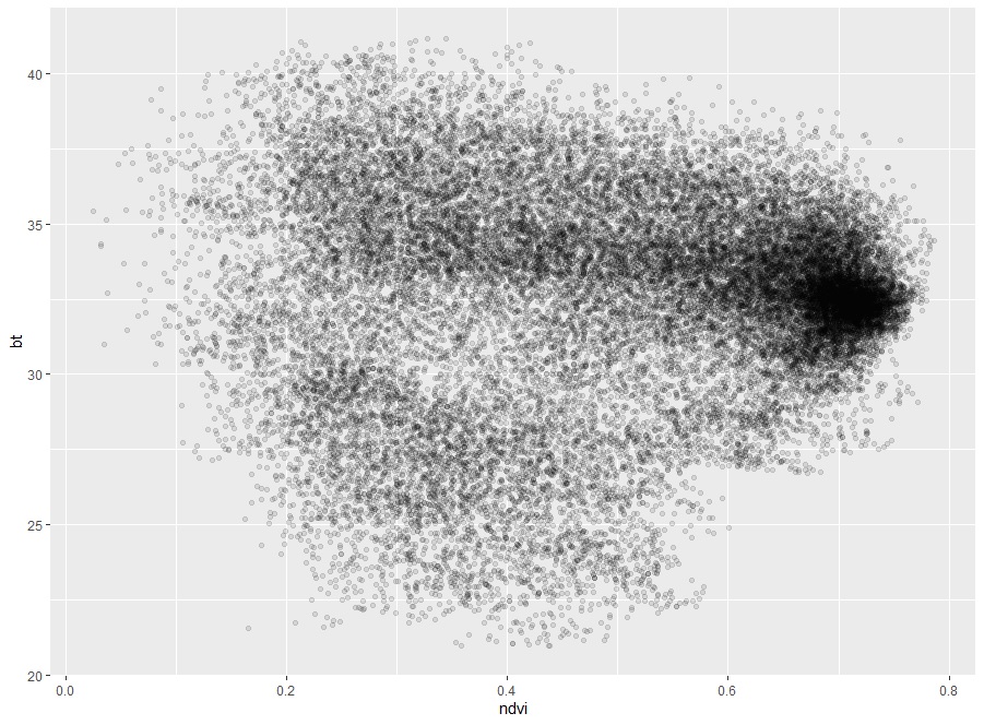
Fig. 5 Scatter plot of NDVI and BT

About Author

Connect with me here.

The media shown in this article are not owned by Analytics Vidhya and is used at the Author’s discretion. 

Rendyk 17 May 2021