Regression Analysis : Real-time Portugal 2019 Election Results

This article was published as a part of the Data Science Blogathon

Hope you all are safe and healthy! Welcome to my blog!

Today, we will see
Regression Analysis using Portugal 2019 Election Results dataset.

Photo by Wojciech Portnicki on Unsplash

Concept :

To give an overview, ML models can be classified based on the task performed and the nature of the output:

Supervised learning under which Regression & Classification comes while in unsupervised learning Clustering is there.

· Regression: Output is a continuous variable.

· Classification: Output is a categorical variable.

· Clustering: No notion of output.

Regression: It is a form of predictive modelling technique where we try to find a significant relationship between a dependent variable and one or more independent variables also called target variables. There are various types of regression techniques: Linear, Logistic, Polynomial, Ridge, Lasso and many more.

About Dataset

This Dataset describes the evolution of results in the Portuguese Parliamentary Elections of October 6th, 2019. The data spans a time interval of 4 hours and 25 minutes, in intervals of 5 minutes, concerning the results of the 27 parties involved in the electoral event.

Dataset has 28 columns in which the “FinalMandates” column is the target variable that describes the number of MPs elected.

The variables in the dataset used: –

1. TimeElapsed (Numeric): Time (minutes) passed since the first data acquisition

2. time (timestamp): Date and time of the data acquisition

3. territoryName (string): Short name of the location (district or nation-wide)

4. totalMandates (numeric): MP’s elected at the moment

5. availableMandates (numeric): MP’s left to elect at the moment

6. numParishes (numeric): Total number of parishes in this location

7. numParishesApproved (numeric): Number of parishes approved in this location

8. blankVotes (numeric): Number of blank votes

9. blankVotesPercentage (numeric): Percentage of blank votes

10. nullVotes (numeric): Number of null votes

11. nullVotesPercentage (numeric): Percentage of null votes

12. votersPercentage (numeric): Percentage of voters

13. subscribedVoters (numeric): Number of subscribed voters in the location

14. totalVoters (numeric): Percentage of blank votes

15. pre.blankVotes (numeric): Number of blank votes (previous election)

16. pre.blankVotesPercentage (numeric): Percentage of blank votes (previous election)

17. pre.nullVotes (numeric): Number of null votes (previous election)

18. pre.nullVotesPercentage (numeric): Percentage of null votes (previous election)

19. pre.votersPercentage (numeric): Percentage of voters (previous election)

20. pre.subscribedVoters (numeric): Number of subscribed voters in the location (previous election)

21. pre.totalVoters (numeric): Percentage of blank votes (previous election)

22. Party (string): Political Party

23. Mandates (numeric): MP’s elected at the moment for the party in a given district

24. Percentage (numeric): Percentage of votes in a party

25. validVotesPercentage (numeric): Percentage of valid votes in a party

26. Votes (numeric): Percentage of party votes

27. Hondt (numeric): Number of MP’s according to the distribution of votes now

28. FinalMandates (numeric): Target: final number of elected MP’s in a district/national level

Here, the task is to predict how many MPs were elected at a district/national level after the 2019 Portugal Parliament Elections.

1. Importing Libraries and Dataset

The first and foremost steps are importing the necessary libraries like NumPy, pandas, matplotlib and seaborn in our notebook.

Then we move on to load the dataset from CSV format and convert it into panda DataFrame and check the top five rows to analyze the data.

2. Cleaning Dataset

1. Checking Null Values: By using dataset isnull().sum() we check that there were no missing values present in the dataset.

2. Checking Datatypes: We checked Datatypes of all columns, to see any inconsistencies in the data.

3. Converting Format: Additionally, in the time column, we’ve changed datatype from object to datetime format for better analysis.

Now conducting EDA to gain insights into the data.

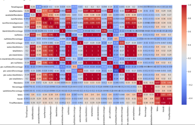
1. Correlation:

Checking correlation with sns.heatmap() revealed that multiple columns are highly correlated.

2. Data Visualization:

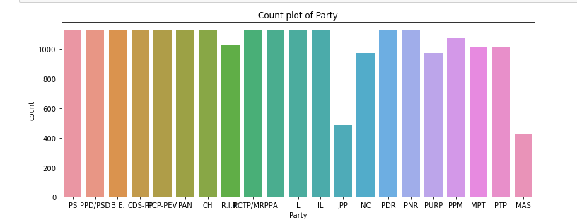
a.  Univariate Analysis:

For this, I plotted countplot for Party and TerritoryName respectively.

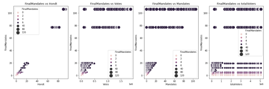
b. Bivariate Analysis:

For bivariate, I plotted different variables against the target
variable-‘Final mandate’ to understand the relationship of the data.

EDA Concluding Remarks:

1. Heatmap Analysis:

we can conclude that many factors have a correlation>0.9 and can be reduced later to reduce the dimensionality of the data.

2. Univariate Data Visualization:

we observe that:

a. Parties with minimum count are JPP and MAS.

b. Most territories have count in the ranges of 800 to 1000 per territory.

3. Bi-Variate Analysis:

We can observe that:

a. Hondt and Votes are directly correlated with the target variable and show discrete values.

b. totalVoters show negligible correlation with the target variable.

c. Party and TerritoryName variables have outliers present in the data.

After the EDA process, we are aware of the changes that need to be incorporated into the dataset to make it more suitable for building machine learning models:

1. PCA (Principal Component Analysis):

As our DataFrame has 28 columns and most of the columns are correlated to a high degree (>0.9), we can use PCA analysis to reduce the dimensionality of the model.

We have divided the variables into two PCA groups based on their correlation: PCA Group A and PCA Group B.

With this analysis we combined the variables into two and columns are reduced from 28 to 15.

2. Label Encoding:

As there are 2 feature variables: TerritoryName and Party, we used Label Encoding to convert them to numerical values.

3. Removing Outliers:

As we observed during Data Visualization that outliers are present in the data. We will further analyze and remove outliers to make the machine learning model more robust.

a. Box Plot:

Box plot was used to further visualize the outliers present in the data for various categorical variables.

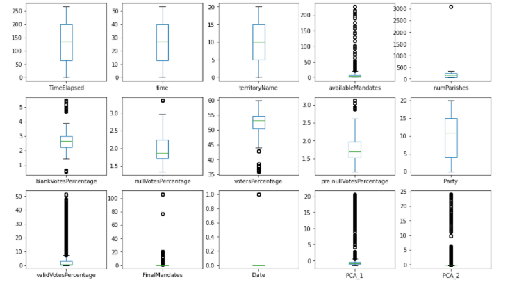
We can observe that many outliers are present in this data and in the next step we will attempt to remove the outliers.

b. Z score Analysis:

This analysis is used to remove outliers from the existing dataset. This analysis works by first calculating z scores for every data value and removing the data with a z score >3.

After applying zscore analysis, we removed around 3299 rows from the dataset. We are currently left with 18344 rows and 15 columns.

c. Normal Distribution Analysis:

To check for normal distribution of the data, first, we plotted Histogram data and checked for skewness.

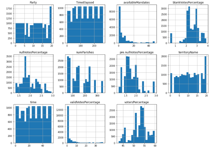
With histplots, we observed that VotersPercantage is skewed towards the left and available Mandates is skewed towards the right. So we converted values from these columns to their sqrt values to normalize the data.

Now, our dataset is ready to be put into the machine learning model for regression analysis.

a. Scaling Dataset:

Standardizing the value of the X variable by using Standard Scaler to make the data normally distributed.

b. Splitting Dataset:

After preprocessing, we now split the data into training/testing subsets.

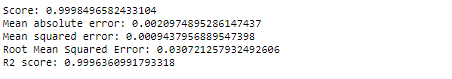
c. Evaluating Models:

We now checked various regression model and calculated metrics such as the model score, Mean Squared Error, Mean Absolute Error, Root Mean Squared Error and R2 Score.

Here, ‘for loop’ is used for fitting different models in one go.

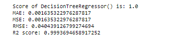
Usually, Mean Squared Error and the R2 Score explain how close the regression line is to the data points. Based on various model performance metrics.

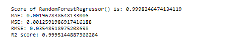
Random Forest Regressor and Decision Tree Regressor performed best with extremely low error and a good R2 score.

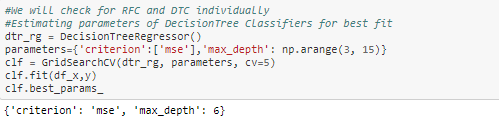
d. Hyper-Parameter Tuning:

Now to increase our accuracy even further, we will perform hyperparameter tuning in both the models and based on final metrics, we will choose the final model.

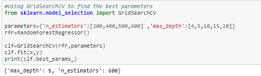
From both the results, Random Forest Regressor is the final model because its RMSE value is smaller RandomForestRegressor( 0.03) than DecisionTreeRegressor(0.04).

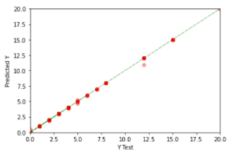
e. Checking Model prediction:

To check model performance, we will now plot a scatter plot between test
results and values predicted by Random Forest-Model.

 

Concluding Remarks

1. Taken output variable as Final Mandate.

2. Understood relationship of target variable with other variables by using Data Visualization:

· Votes, Hondt have a linear positive relationship.

· Total Votes, Mandates have discreet values against Target variable.

· Correlation between many variables >0.9, hence used PCA to decrease the dimensionality of the data from 28 to 17.

· Label Encoded object data such as Party and territory Name for better EDA analysis.

3. Removed outliers using z score analysis and converted data into a normal distribution.

4. Checked various regressor models and found Random Forest and Decision Tree with best R2score values>0.99

5. Performed hyper-tuning to find the best parameters of these models and finally chose Random Forest for the final model.

6. Final score for RFR model is 0.9998, RMSE is 0.02 and the R2 score is 0.9996.

7. Plotted to scatter plot and found a linear line that shows a close match between test and predicted values.

8. Overall, the model is a good predictor of true values.

Here is the link to my complete solution and dataset used:

https://github.com/priyalagarwal27/Regression-on-ELECTION-dataset

Well, What are your thoughts on this? I would love to hear yours. I hope you liked the article.

Stay connected for more related articles. Please leave any suggestions, questions, requests for further clarifications down below in the comment section.

Thanks for the reading and Happy Machine Learning!!!

The media shown in this article are not owned by Analytics Vidhya and is used at the Author’s discretion.

Priyal Agarwal 23 May 2021

My name is Priyal Agarwal. Recently I've completed a PG program in data science, Machine Learning, and neural networks and I've experienced as a data science intern in Fliprobo technologies, Bangalore as well. I am an enthusiastic, self-motivated, reliable, dedicated and open- minded person. I get across to people and adjust to changes with ease. I believe that a person should work on developing their professional skills and learning new things all the time. For that, I write technical blogs/articles on medium and Analytics Vidhya in contribution to the Data Science Community and learn about new technologies to excel my knowledge.