A Gentle Introduction to Autoencoders for Data Science Enthusiasts

This article was published as a part of the Data Science Blogathon

“A breakthrough in machine learning would be worth ten Microsofts“— Bill Gates

Introduction

In the era of Artificial Intelligence (AI), human efforts are minimized by applying automation to several processes. As technology is increasing storage and computation capabilities are also increasing, as we all know Deep Learning and Machine Learning concepts are around us almost since 60 Years back but due to the lack of these resources, we were not able to explore these technologies much.

In the past few years, we have seen a boom in the field of AI, it is being applied to multiple fields like Healthcare, Insurance, Banking, etc. This was all possible because we have good GPUs and Faster Storage mechanisms.

Now you might be wondering why am I talking about the storage and processing capabilities of the AI while I should be discussing what are Autoencoders right? So storage is specifically what makes Autoencoders prominent in Machine Learning. Autoencoders are the self-supervised models that can learn to compress the input data efficiently. Although this is not the only use-case of Autoencoders there are plenty. So first let’s discuss what is Autoencoder.

What are Autoencoders ?

Autoencoders are self-supervised machine learning models which are used to reduce the size of input data by recreating it. These models are trained as supervised machine learning models and during inference, they work as unsupervised models that’s why they are called self-supervised models. Autoencoder is made up of two components:

1. Encoder: It works as a compression unit that compresses the input data.

2. Decoder: It decompresses the compressed input by reconstructing it.

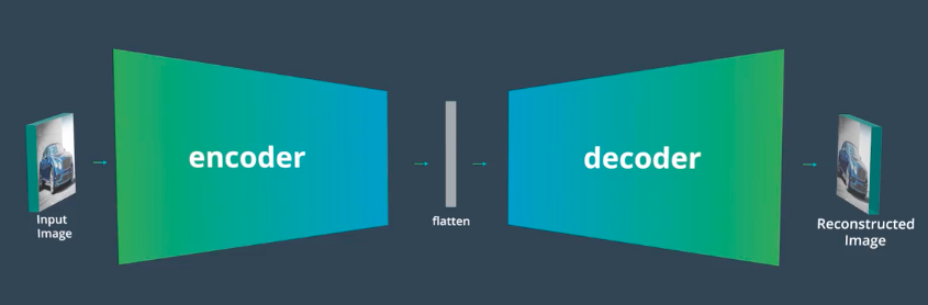
In an Autoencoder both Encoder and Decoder are made up of a combination of NN (Neural Networks) layers, which helps to reduce the size of the input image by recreating it. In the case of CNN Autoencoder, these layers are CNN layers (Convolutional, Max Pool, Flattening, etc.) while in the case of RNN/LSTM their respective layers are used.

Applications of Autoencoders

Three are several applications of Autoencoders some of the important ones are:

1. File Compression: Primary use of Autoencoders is that they can reduce the dimensionality of input data which we in common refer to as file compression. Autoencoders works with all kinds of data like Images, Videos, and Audio, this helps in sharing and viewing data faster than we could do with its original file size.

2. Image De-noising: Autoencoders are also used as noise removal techniques (Image De-noising), what makes it the best choice for De-noising is that it does not require any human interaction, once trained on any kind of data it can reproduce that data with less noise than the original image.

3. Image Transformation: Autoencoders are also used for image transformations, which is typically classified under GAN(Generative Adversarial Networks) models. Using these we can transform B/W images to colored one and vice versa, we can up-sample and down-sample the input data, etc.

Create a Simple Autoencoder for Image File Compression

Using Autoencoders we can compress image files which are great for sharing and saving in a faster and more memory efficient way. These compressed images contain the key information same as in original images but in a compressed format that can be used further for other reconstructions and transformations.

We will create a simple Autoencoder that can compress the image file for the MNIST dataset, by using the following mechanism:

For creating the Autoencoder we will use Python language and Torch framework.

Let’s start by importing the required libraries and MNIST dataset on which we want to apply compression.

import torch
import numpy as np
from torchvision import datasets
import torchvision.transforms as transforms
# convert data to torch.FloatTensor
transform = transforms.ToTensor()
# load the training and test datasets
train_data = datasets.MNIST(root='data', train=True,
                                   download=True, transform=transform)
test_data = datasets.MNIST(root='data', train=False,
                                  download=True, transform=transform)

We have imported torch for defining Autoencoder, NumPy for scientific computations, datasets from torchvision for reading the MNIST dataset, and finally transforms function for converting variables to torch tensors, which is required format while working with torch library.

# Create training and test dataloaders
# number of subprocesses to use for data loading
num_workers = 0
# how many samples per batch to load
batch_size = 20
# prepare data loaders
train_loader = torch.utils.data.DataLoader(train_data, batch_size=batch_size, num_workers=num_workers)
test_loader = torch.utils.data.DataLoader(test_data, batch_size=batch_size, num_workers=num_workers)

After loading data, we will create loader functions for training and testing our model, for visualization we can use the following code segment:

import matplotlib.pyplot as plt
%matplotlib inline
# obtain one batch of training images
dataiter = iter(train_loader)
images, labels = dataiter.next()
images = images.numpy()
# get one image from the batch
img = np.squeeze(images[0])
fig = plt.figure(figsize = (5,5)) 
ax = fig.add_subplot(111)
ax.imshow(img, cmap='gray')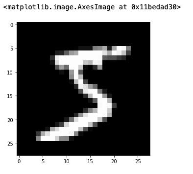

After visualization, now is the time of defining the Encoder and Decoder functions for Autoencoder. We are going to flatten the input matrix to a size of 784 length vector. Images in the MNIST dataset have pixel values of only 0 (black) or 255 (white).

We going to make use of only flattening layers because of which this is often called a Linear Autoencoder, Activation functions that we will be using are Relu at the input end and Sigmoid at the output end. We are making use of Sigmoid because the output that we want is made up of only 0 and 255 (0 and 1 values) which is obtained by Sigmoid only.

import torch.nn as nn
import torch.nn.functional as F
# define the NN architecture
class Autoencoder(nn.Module):
    def __init__(self, encoding_dim):
        super(Autoencoder, self).__init__()
        ## encoder ##
        # linear layer (784 -> encoding_dim)
        self.fc1 = nn.Linear(28 * 28, encoding_dim)
        ## decoder ##
        # linear layer (encoding_dim -> input size)
        self.fc2 = nn.Linear(encoding_dim, 28*28)
    def forward(self, x):
        # add layer, with relu activation function
        x = F.relu(self.fc1(x))
        # output layer (sigmoid for scaling from 0 to 1)
        x = F.sigmoid(self.fc2(x))
        return x
# initialize the NN
encoding_dim = 32
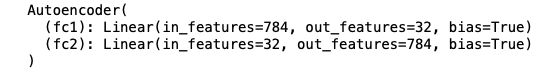
model = Autoencoder(encoding_dim)
print(model)

For the training of the torch model, we need to create a class first, for this model we have created a class named Autoencoder, in which we have created two linear (flattening) layers fc1 and fc2. The first layer fc1 works as an Encoder and compresses the input image to (784, 32) dimension vector, and the second layer fc2 works as a Decoder and decompresses the image to (32, 784) dimension, which is the required output dimension. The output of the above code segment looks like this:

After defining Encoder and Decoder, we will have to decide the optimizer and loss function for training the model.

# specify loss function
criterion = nn.MSELoss()
# specify loss function
optimizer = torch.optim.Adam(model.parameters(), lr=0.001)

For this linear Autoencoder, we are going to use MSE (Mean Squared Error Loss) and Adam optimizer.

Training the model works as follows:

1. Pass the input image to the model and generate the output using the Sigmoid activation function.

2. Calculate the loss of actual and predicted values.

3. Backpropagate and adjust the parameters in order to minimize the loss.

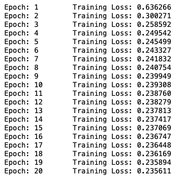
# number of epochs to train the model
n_epochs = 20
for epoch in range(1, n_epochs+1):
    # monitor training loss
    train_loss = 0.0
    ###################
    # train the model #
    ###################
    for data in train_loader:
        # _ stands in for labels, here
        images, _ = data
        # flatten images
        images = images.view(images.size(0), -1)
        # clear the gradients of all optimized variables
        optimizer.zero_grad()
        # forward pass: compute predicted outputs by passing inputs to the model
        outputs = model(images)
        # calculate the loss
        loss = criterion(outputs, images)
        # backward pass: compute gradient of the loss with respect to model parameters
        loss.backward()
        # perform a single optimization step (parameter update)
        optimizer.step()
        # update running training loss
        train_loss += loss.item()*images.size(0)
    # print avg training statistics 
    train_loss = train_loss/len(train_loader)
    print('Epoch: {} tTraining Loss: {:.6f}'.format(
        epoch, 
        train_loss ))

Above is the code for training the Autoencoder model using those mentioned steps. The output of the code would look something like this:

Once the model is trained we can use the following model for inferencing.

# obtain one batch of test images
dataiter = iter(test_loader)
images, labels = dataiter.next()
images_flatten = images.view(images.size(0), -1)
# get sample outputs
output = model(images_flatten)
# prep images for display
images = images.numpy()
# output is resized into a batch of images
output = output.view(batch_size, 1, 28, 28)
# use detach when it's an output that requires_grad
output = output.detach().numpy()
# plot the first ten input images and then reconstructed images
fig, axes = plt.subplots(nrows=2, ncols=10, sharex=True, sharey=True, figsize=(25,4))
# input images on top row, reconstructions on bottom
for images, row in zip([images, output], axes):
    for img, ax in zip(images, row):
        ax.imshow(np.squeeze(img), cmap='gray')
        ax.get_xaxis().set_visible(False)
        ax.get_yaxis().set_visible(False)

The output that you would get while inferencing would look something like this.

So this is how you can create your own image compressor using Autoencoders. This can be done for any image dataset. Currently, we have made use of only linear layers but CNN and LSTM layers can also be used in order o improve the quality of compression while preserving the key data, but that is for the next lecture.

References

Udacity Deep Learning: https://www.udacity.com/

Thanks for reading this article do like if you have learned something new, feel free to comment See you next time !!! ❤️

The media shown in this article are not owned by Analytics Vidhya and are used at the Author’s discretion.