Complete guide on How to use Autoencoders in Python
This article was published as a part of the Data Science Blogathon
Introduction
An autoencoder is actually an Artificial Neural Network that is used to decompress and compress the input data provided in an unsupervised manner. Decompression and compression operations are lossy and data-specific.
Data specific means that the autoencoder will only be able to actually compress the data on which it has been trained. For example, if you train an autoencoder with images of dogs, then it will give a bad performance for cats. The autoencoder plans to learn the representation which is known as the encoding for a whole set of data. This can result in the reduction of the dimensionality by the training network. The reconstruction part is also learned with this.
Lossy operations mean that the reconstructed image is often not an as sharp or high resolution in quality as the original one and the difference is greater for reconstructions with a greater loss and this is known as a lossy operation. The following image shows how the image is encoded and decoded with a certain loss factor.
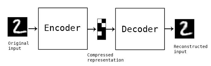
The Autoencoder is a particular type of feed-forward neural network and the input should be similar to the output. Hence we would need an encoding method, loss function, and a decoding method. The end goal is to perfectly replicate the input with minimum loss.
The Input will be passed through a layer of encoders which are actually a fully connected neural network that also makes the code decoder and hence use the same code for encoding and decoding like an ANN.
Code Implementation
A Trained ANN through backpropagation works in the same way as the autoencoders. In this article we are going to discuss 3 types of autoencoders which are as follows :
-
Simple autoencoder
-
Deep CNN autoencoder
-
Denoising autoencoder
For the implementation part of the autoencoder, we will use the popular MNIST dataset of digits.
1. Simple Autoencoder
We begin by importing all the necessary libraries :
import all the dependencies
from keras.layers import Dense,Conv2D,MaxPooling2D,UpSampling2D
from keras import Input, Model
from keras.datasets import mnist
import numpy as np
import matplotlib.pyplot as plt
Then we will build our model and we will provide the number of dimensions that will decide how much the input will be compressed. The lesser the dimension, the more will be the compression.
encoding_dim = 15
input_img = Input(shape=(784,))
# encoded representation of input
encoded = Dense(encoding_dim, activation='relu')(input_img)
# decoded representation of code
decoded = Dense(784, activation='sigmoid')(encoded)
# Model which take input image and shows decoded images
autoencoder = Model(input_img, decoded)
Then we need to build the encoder model and decoder model separately so that we can easily differentiate between the input and output.
# This model shows encoded images
encoder = Model(input_img, encoded)
# Creating a decoder model
encoded_input = Input(shape=(encoding_dim,))
# last layer of the autoencoder model
decoder_layer = autoencoder.layers[-1]
# decoder model
decoder = Model(encoded_input, decoder_layer(encoded_input))
Then we need to compile the model with the ADAM optimizer and cross-entropy loss function fitment.
autoencoder.compile(optimizer='adam', loss='binary_crossentropy')
Then you need to load the data :
(x_train, y_train), (x_test, y_test) = mnist.load_data()
x_train = x_train.astype('float32') / 255.
x_test = x_test.astype('float32') / 255.
x_train = x_train.reshape((len(x_train), np.prod(x_train.shape[1:])))
x_test = x_test.reshape((len(x_test), np.prod(x_test.shape[1:])))
print(x_train.shape)
print(x_test.shape)
Output :
(60000, 784)
(10000, 784)
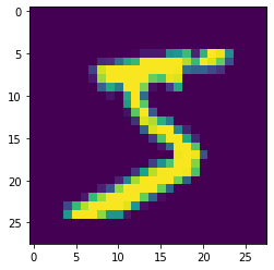
If you want to see how the data is actually, you can use the following line of code :
plt.imshow(x_train[0].reshape(28,28))
Output :
Then you need to train your model :
autoencoder.fit(x_train, x_train,
                epochs=15,
                batch_size=256,
                validation_data=(x_test, x_test))
Output :
Epoch 1/15
235/235 [==============================] - 14s 5ms/step - loss: 0.4200 - val_loss: 0.2263
Epoch 2/15
235/235 [==============================] - 1s 3ms/step - loss: 0.2129 - val_loss: 0.1830
Epoch 3/15
235/235 [==============================] - 1s 3ms/step - loss: 0.1799 - val_loss: 0.1656
Epoch 4/15
235/235 [==============================] - 1s 3ms/step - loss: 0.1632 - val_loss: 0.1537
Epoch 5/15
235/235 [==============================] - 1s 3ms/step - loss: 0.1533 - val_loss: 0.1481
Epoch 6/15
235/235 [==============================] - 1s 3ms/step - loss: 0.1488 - val_loss: 0.1447
Epoch 7/15
235/235 [==============================] - 1s 3ms/step - loss: 0.1457 - val_loss: 0.1424
Epoch 8/15
235/235 [==============================] - 1s 3ms/step - loss: 0.1434 - val_loss: 0.1405
Epoch 9/15
235/235 [==============================] - 1s 3ms/step - loss: 0.1415 - val_loss: 0.1388
Epoch 10/15
235/235 [==============================] - 1s 3ms/step - loss: 0.1398 - val_loss: 0.1374
Epoch 11/15
235/235 [==============================] - 1s 3ms/step - loss: 0.1386 - val_loss: 0.1360
Epoch 12/15
235/235 [==============================] - 1s 3ms/step - loss: 0.1373 - val_loss: 0.1350
Epoch 13/15
235/235 [==============================] - 1s 3ms/step - loss: 0.1362 - val_loss: 0.1341
Epoch 14/15
235/235 [==============================] - 1s 3ms/step - loss: 0.1355 - val_loss: 0.1334
Epoch 15/15
235/235 [==============================] - 1s 3ms/step - loss: 0.1348 - val_loss: 0.1328
After training, you need to provide the input and you can plot the results using the following code :
encoded_img = encoder.predict(x_test)
decoded_img = decoder.predict(encoded_img)
plt.figure(figsize=(20, 4))
for i in range(5):
    # Display original
    ax = plt.subplot(2, 5, i + 1)
    plt.imshow(x_test[i].reshape(28, 28))
    plt.gray()
    ax.get_xaxis().set_visible(False)
    ax.get_yaxis().set_visible(False)
    # Display reconstruction
    ax = plt.subplot(2, 5, i + 1 + 5)
    plt.imshow(decoded_img[i].reshape(28, 28))
    plt.gray()
    ax.get_xaxis().set_visible(False)
    ax.get_yaxis().set_visible(False)
plt.show()
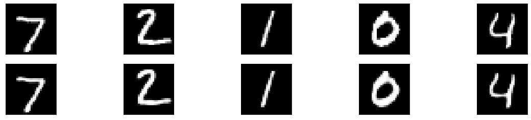
You can clearly see the output for the encoded and decoded images respectively as shown below.
2. Deep CNN Autoencoder :
Since the input here is images, it does make more sense to use a Convolutional Neural network or CNN. The encoder will be made up of a stack of Conv2D and max-pooling layer and the decoder will have a stack of Conv2D and Upsampling Layer.
Code :
model = Sequential()
# encoder network
model.add(Conv2D(30, 3, activation= 'relu', padding='same', input_shape = (28,28,1)))
model.add(MaxPooling2D(2, padding= 'same'))
model.add(Conv2D(15, 3, activation= 'relu', padding='same'))
model.add(MaxPooling2D(2, padding= 'same'))
#decoder network
model.add(Conv2D(15, 3, activation= 'relu', padding='same'))
model.add(UpSampling2D(2))
model.add(Conv2D(30, 3, activation= 'relu', padding='same'))
model.add(UpSampling2D(2))
model.add(Conv2D(1,3,activation='sigmoid', padding= 'same')) # output layer
model.compile(optimizer= 'adam', loss = 'binary_crossentropy')
model.summary()
Output :
Model: "sequential"
_________________________________________________________________
Layer (type)                 Output Shape              Param #
=================================================================
conv2d (Conv2D)              (None, 28, 28, 30)        300
_________________________________________________________________
max_pooling2d (MaxPooling2D) (None, 14, 14, 30)        0
_________________________________________________________________
conv2d_1 (Conv2D)            (None, 14, 14, 15)        4065
_________________________________________________________________
max_pooling2d_1 (MaxPooling2 (None, 7, 7, 15)          0
_________________________________________________________________
conv2d_2 (Conv2D)            (None, 7, 7, 15)          2040
_________________________________________________________________
up_sampling2d (UpSampling2D) (None, 14, 14, 15)        0
_________________________________________________________________
conv2d_3 (Conv2D)            (None, 14, 14, 30)        4080
_________________________________________________________________
up_sampling2d_1 (UpSampling2 (None, 28, 28, 30)        0
_________________________________________________________________
conv2d_4 (Conv2D)            (None, 28, 28, 1)         271
=================================================================
Total params: 10,756
Trainable params: 10,756
Non-trainable params: 0
_________________________________________________________________
Now you need to load the data and training the model
(x_train, _), (x_test, _) = mnist.load_data()
x_train = x_train.astype('float32') / 255.
x_test = x_test.astype('float32') / 255.
x_train = np.reshape(x_train, (len(x_train), 28, 28, 1))
x_test = np.reshape(x_test, (len(x_test), 28, 28, 1))
model.fit(x_train, x_train,
                epochs=15,
                batch_size=128,
                validation_data=(x_test, x_test))
Output :
Epoch 1/15
469/469 [==============================] - 34s 8ms/step - loss: 0.2310 - val_loss: 0.0818
Epoch 2/15
469/469 [==============================] - 3s 7ms/step - loss: 0.0811 - val_loss: 0.0764
Epoch 3/15
469/469 [==============================] - 3s 7ms/step - loss: 0.0764 - val_loss: 0.0739
Epoch 4/15
469/469 [==============================] - 3s 7ms/step - loss: 0.0743 - val_loss: 0.0725
Epoch 5/15
469/469 [==============================] - 3s 7ms/step - loss: 0.0729 - val_loss: 0.0718
Epoch 6/15
469/469 [==============================] - 3s 7ms/step - loss: 0.0722 - val_loss: 0.0709
Epoch 7/15
469/469 [==============================] - 3s 7ms/step - loss: 0.0715 - val_loss: 0.0703
Epoch 8/15
469/469 [==============================] - 3s 7ms/step - loss: 0.0709 - val_loss: 0.0698
Epoch 9/15
469/469 [==============================] - 3s 7ms/step - loss: 0.0700 - val_loss: 0.0693
Epoch 10/15
469/469 [==============================] - 3s 7ms/step - loss: 0.0698 - val_loss: 0.0689
Epoch 11/15
469/469 [==============================] - 3s 7ms/step - loss: 0.0694 - val_loss: 0.0687
Epoch 12/15
469/469 [==============================] - 3s 7ms/step - loss: 0.0691 - val_loss: 0.0684
Epoch 13/15
469/469 [==============================] - 3s 7ms/step - loss: 0.0688 - val_loss: 0.0680
Epoch 14/15
469/469 [==============================] - 3s 7ms/step - loss: 0.0685 - val_loss: 0.0680
Epoch 15/15
469/469 [==============================] - 3s 7ms/step - loss: 0.0683 - val_loss: 0.0676
Now you need to provide the input and plot the output for the following results
pred = model.predict(x_test)
plt.figure(figsize=(20, 4))
for i in range(5):
    # Display original
    ax = plt.subplot(2, 5, i + 1)
    plt.imshow(x_test[i].reshape(28, 28))
    plt.gray()
    ax.get_xaxis().set_visible(False)
    ax.get_yaxis().set_visible(False)
    # Display reconstruction
    ax = plt.subplot(2, 5, i + 1 + 5)
    plt.imshow(pred[i].reshape(28, 28))
    plt.gray()
    ax.get_xaxis().set_visible(False)
    ax.get_yaxis().set_visible(False)
plt.show()
Output :
3. Denoising Autoencoder
Now we will see how the model performs with noise in the image. What we mean by noise is blurry images, changing the color of the images, or even white markers on the image.
noise_factor = 0.7
x_train_noisy = x_train + noise_factor * np.random.normal(loc=0.0, scale=1.0, size=x_train.shape)
x_test_noisy = x_test + noise_factor * np.random.normal(loc=0.0, scale=1.0, size=x_test.shape)
x_train_noisy = np.clip(x_train_noisy, 0., 1.)
x_test_noisy = np.clip(x_test_noisy, 0., 1.)
Here is how the noisy images look right now.
plt.figure(figsize=(20, 2))
for i in range(1, 5 + 1):
    ax = plt.subplot(1, 5, i)
    plt.imshow(x_test_noisy[i].reshape(28, 28))
    plt.gray()
    ax.get_xaxis().set_visible(False)
    ax.get_yaxis().set_visible(False)
plt.show()
Output :
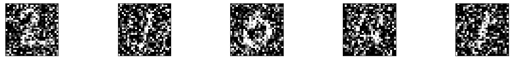
Now the images are barely identifiable and to increase the extent of the autoencoder, we will modify the layers of the defined model to increase the filter so that the model performs better and then fit the model.
model = Sequential()
# encoder network
model.add(Conv2D(35, 3, activation= 'relu', padding='same', input_shape = (28,28,1)))
model.add(MaxPooling2D(2, padding= 'same'))
model.add(Conv2D(25, 3, activation= 'relu', padding='same'))
model.add(MaxPooling2D(2, padding= 'same'))
#decoder network
model.add(Conv2D(25, 3, activation= 'relu', padding='same'))
model.add(UpSampling2D(2))
model.add(Conv2D(35, 3, activation= 'relu', padding='same'))
model.add(UpSampling2D(2))
model.add(Conv2D(1,3,activation='sigmoid', padding= 'same')) # output layer
model.compile(optimizer= 'adam', loss = 'binary_crossentropy')
model.fit(x_train_noisy, x_train,
                epochs=15,
                batch_size=128,
                validation_data=(x_test_noisy, x_test))
Output :
Epoch 1/15
469/469 [==============================] - 5s 9ms/step - loss: 0.2643 - val_loss: 0.1456
Epoch 2/15
469/469 [==============================] - 4s 8ms/step - loss: 0.1440 - val_loss: 0.1378
Epoch 3/15
469/469 [==============================] - 4s 8ms/step - loss: 0.1373 - val_loss: 0.1329
Epoch 4/15
469/469 [==============================] - 4s 8ms/step - loss: 0.1336 - val_loss: 0.1305
Epoch 5/15
469/469 [==============================] - 4s 8ms/step - loss: 0.1313 - val_loss: 0.1283
Epoch 6/15
469/469 [==============================] - 4s 8ms/step - loss: 0.1294 - val_loss: 0.1268
Epoch 7/15
469/469 [==============================] - 4s 8ms/step - loss: 0.1278 - val_loss: 0.1257
Epoch 8/15
469/469 [==============================] - 4s 8ms/step - loss: 0.1267 - val_loss: 0.1251
Epoch 9/15
469/469 [==============================] - 4s 8ms/step - loss: 0.1259 - val_loss: 0.1244
Epoch 10/15
469/469 [==============================] - 4s 8ms/step - loss: 0.1251 - val_loss: 0.1234
Epoch 11/15
469/469 [==============================] - 4s 8ms/step - loss: 0.1241 - val_loss: 0.1234
Epoch 12/15
469/469 [==============================] - 4s 8ms/step - loss: 0.1239 - val_loss: 0.1222
Epoch 13/15
469/469 [==============================] - 4s 8ms/step - loss: 0.1232 - val_loss: 0.1223
Epoch 14/15
469/469 [==============================] - 4s 8ms/step - loss: 0.1226 - val_loss: 0.1215
Epoch 15/15
469/469 [==============================] - 4s 8ms/step - loss: 0.1221 - val_loss: 0.1211
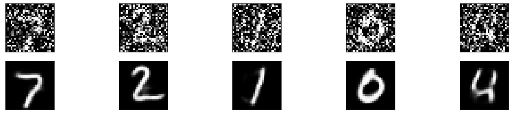
After the training, we will provide the input and write a plot function to see the final results.
pred = model.predict(x_test_noisy)
plt.figure(figsize=(20, 4))
for i in range(5):
    # Display original
    ax = plt.subplot(2, 5, i + 1)
    plt.imshow(x_test_noisy[i].reshape(28, 28))
    plt.gray()
    ax.get_xaxis().set_visible(False)
    ax.get_yaxis().set_visible(False)
    # Display reconstruction
    ax = plt.subplot(2, 5, i + 1 + 5)
    plt.imshow(pred[i].reshape(28, 28))
    plt.gray()
    ax.get_xaxis().set_visible(False)
    ax.get_yaxis().set_visible(False)
plt.show()
Output :
Endnotes :
We have gone through the structure of how autoencoders work and worked with 3 types of autoencoders. There are multiple uses for autoencoders like dimensionality reduction image compression, recommendations system for movies and songs and more. The performance of the model can be increased by training it for more epochs or also by increasing the dimension of our network.
Thank you for reading till the end. Hope you are doing well and stay safe and are getting vaccinated soon or already are.
About the Author :
Data Engineer | Python, C/C++, AWS Developer | Freelance Tech Writer
Just a guy who loves to code and learn new languages and concepts


Thank you concept is well explained.