Complete Guide to Moment Generating Functions in Statistics For Data Science

Introduction

When it comes to statistical moments like mean, variance, and skewness, understanding Moment-Generating Functions (MGF) is essential, whether you’re dealing with continuous or discrete probability distributions. In this article, we’ll explore how to find Moment Generating Functions, breaking down their concepts and showing how they’re used in real-life situations through practical examples. So, let’s dive in and discover the role of moment-generating function in data science!

This article was published as a part of the Data Science Blogathon.

What are Statistical Moments?

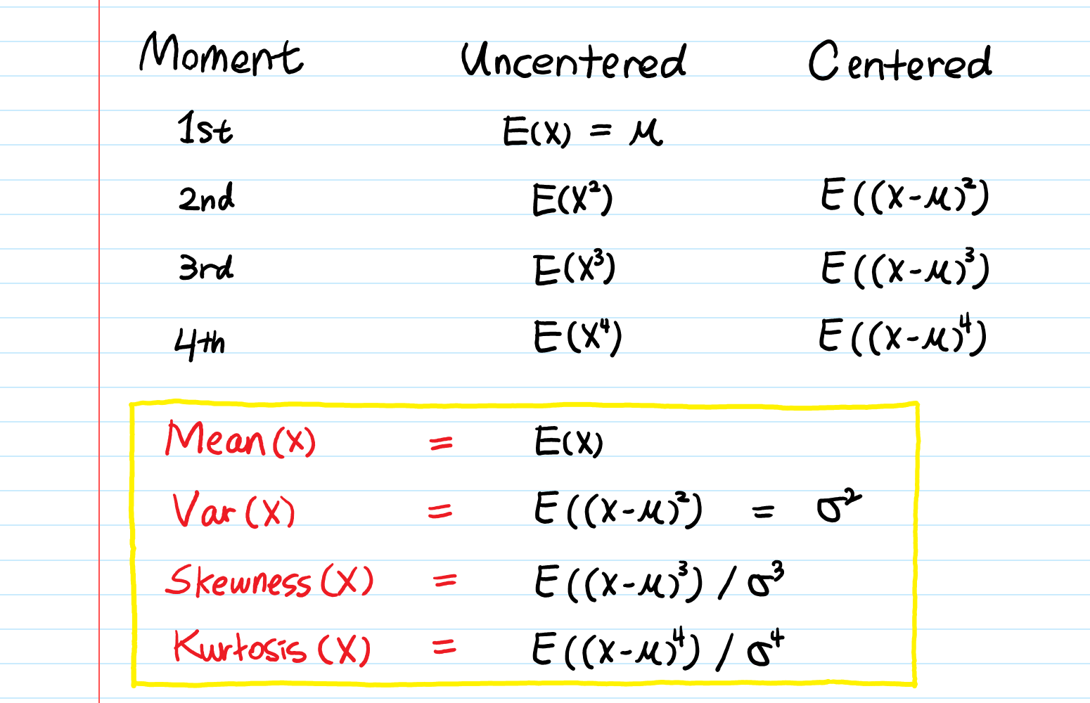
Statistical moments provide insights into random variables like X. Moments are essentially expected values, such as E(X), E(X²), E(X³), and so on. These moments have specific names:

• The first moment is E(X).
• The second moment is E(X²).
• The third moment is E(X³).
• And so on, up to the n-th moment, which is E(Xⁿ).

In statistics, we commonly encounter the first two moments:

• Mean (μ) = E(X): It represents the average value.
• Variance (σ²) = E(X²) – (E(X))² = E(X²) − μ²: It quantifies the spread of data around the mean.

While mean and variance are crucial for understanding a random variable, there are other moments worth exploring. For instance, the third moment, E(X³), indicates skewness, revealing distribution asymmetry. The fourth moment, E(X⁴), relates to kurtosis, providing insights into the distribution’s tail behavior. These additional characteristics help define probability distributions more comprehensively.

What is the Moment Generating Function?

The moment-generating function (MGF) associated with a random variable X, is a function,

M_X : R → [0,∞] defined by:

 M_X(t) = E [ e^tX ]

The domain or region of convergence (ROC) of M_X is the set D_X = { t | M_X(t) < ∞}.

In general, t can be a complex number, but since we did not define the expectations for complex-valued random variables, so we will restrict ourselves only to real-valued t. And the point to note that t= 0 is always a point in the ROC for any random variable since M_X (0) = 1.

As its name implies, MGF is the function that generates the moments:

E(X), E(X²), E(X³), …, E(Xⁿ)

Cases

If X is discrete with probability mass function(pmf) p_X (x), then

M_X (t) = Σ e^tx p_X (x)

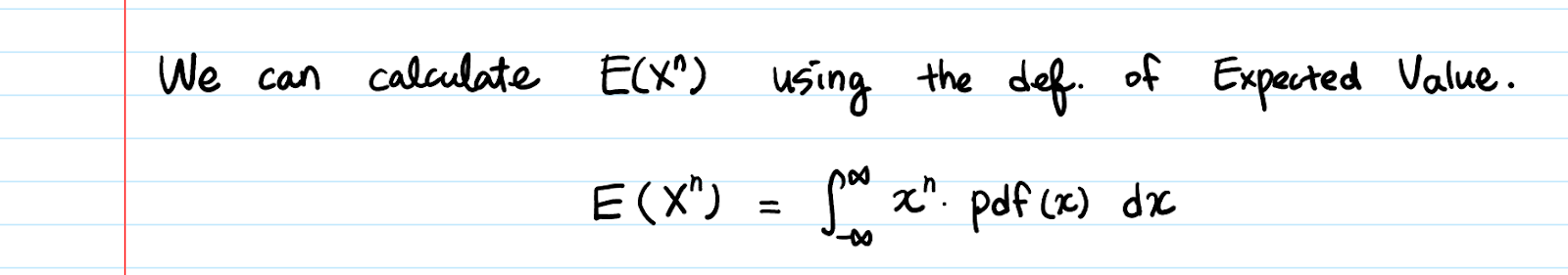
If X is continuous with probability density function (pdf) f_X (x), then:

 M_X (t) = ∫ e^tx f_X (x) dx

How to Find Moment Generating Functions

Moment Generating Functions (MGFs) is crucial in the realm of probability theory and statistics. MGFs provide a powerful tool for analyzing random variables, enabling us to derive moments and probability distributions with ease. In this guide, we’ll walk you through the process of finding MGFs step by step, equipping you with the knowledge to tackle any probability problem confidently.

Step 1: Definition of Moment Generating Functions

The Moment Generating Function of a random variable X, denoted by M(t), is defined as the expected value of e^(tX), where t is a parameter:
M(t) = E(e^(tX)

Step 2: Steps to Find MGFs

1. Start with the probability distribution function (pdf) or probability mass function (pmf) of the random variable X.
2. Replace X in the pdf or pmf with tx, where t is the parameter.
3. Calculate the expected value of e^(tx).
4. Simplify the expression to obtain the MGF, M(t).

Step 3: Example Calculation

Let’s consider a simple example of finding the MGF of a Poisson random variable with parameter λ.

1. Start with the pmf of the Poisson distribution: P(X=k) = (e^(-λ) * λ^k) / k!
2. Replace X with tx: P(tx=k) = (e^(-λ) * (λt)^k) / k!
3. Calculate the expected value: M(t) = E(e^(tx)) = Σ(e^(tx) * P(tx=k)) for all possible values of k.
4. Simplify the expression to obtain the MGF of the Poisson distribution.

Step 4: Properties of MGFs

MGFs possess several important properties:

• Uniqueness: Two random variables with the same MGF have the same distribution.
• Moments: Derivatives of the MGF provide moments of the random variable.
• Cumulants: Logarithms of the MGF provide cumulants, which are useful in characterizing distributions.

Step 5: Applications of MGFs

MGFs find applications in various fields, including finance, physics, and engineering. They enable us to analyze the behavior of random variables and make predictions with statistical accuracy.

Properties of Moment Generating Functions

1. Condition for a Valid MGF:

M_X(0) = 1 i.e, Whenever you compute an MGF, plug in t = 0 and see if you get 1.

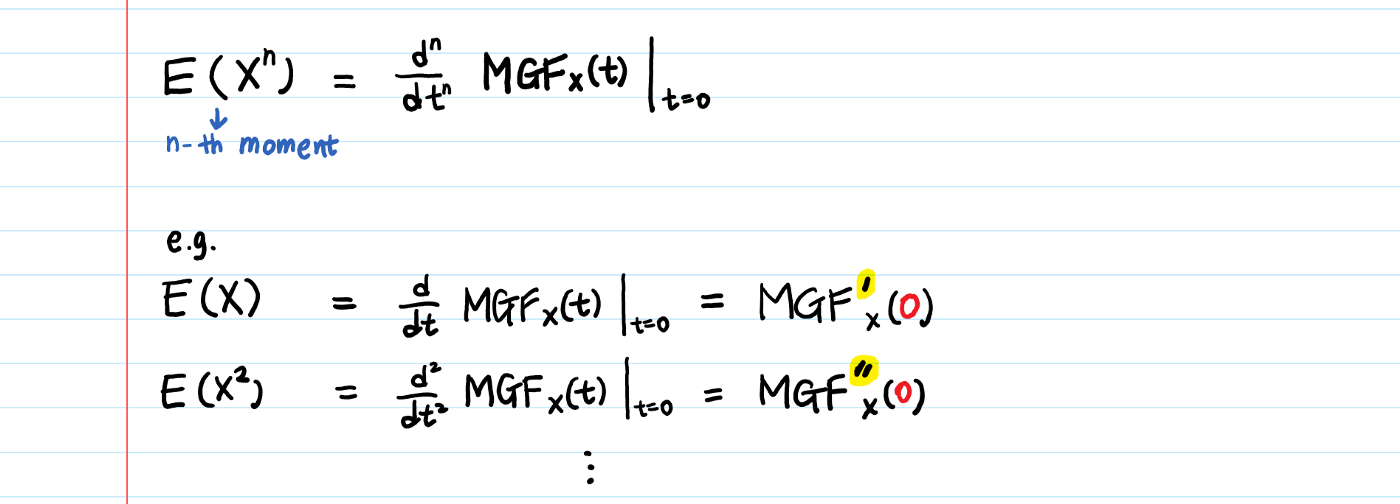
2. Moment Generating Property:

By looking at the definition of MGF, we might think that how we formulate it in the form of E(Xⁿ) instead of E(e^tx). 

So, to do this we take a derivative of MGF n times and plug t = 0 in. then, you will get E(Xⁿ).

Proof

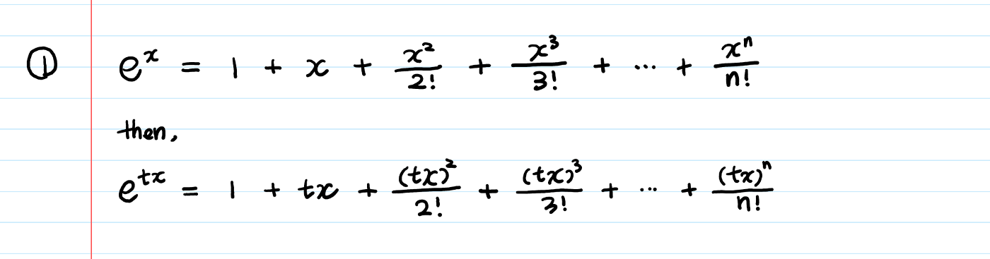
To prove the above property, we take the help of Taylor’s Series:

Step-1: Let’s see Taylor’s series Expansion of e^X and then by using that expansion, we generate the expansion for e^tX which we will use in later steps.

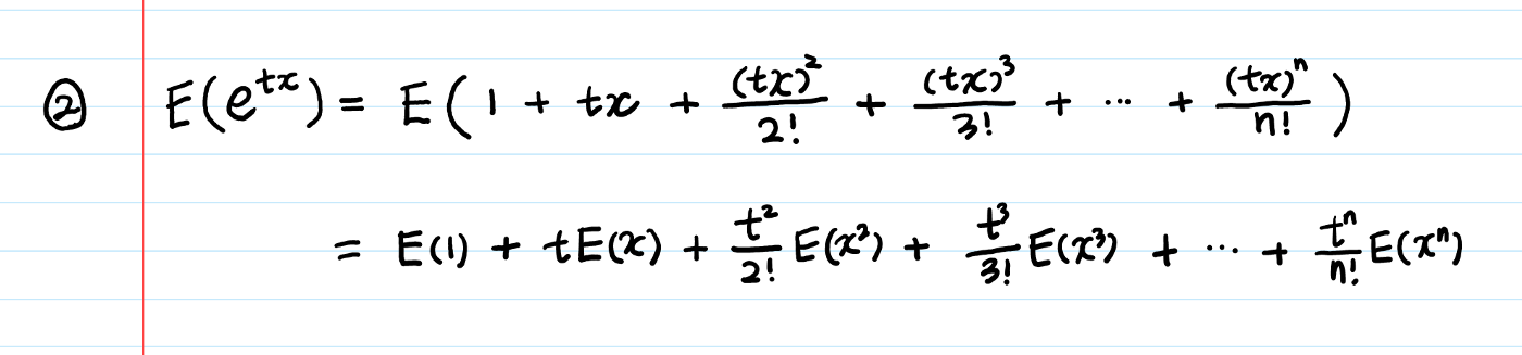
Step-2: Take the expectation on both sides of the equation, we get:

Step-3: Now, take the derivative of the equation with respect to t and then we will reach our conclusion.

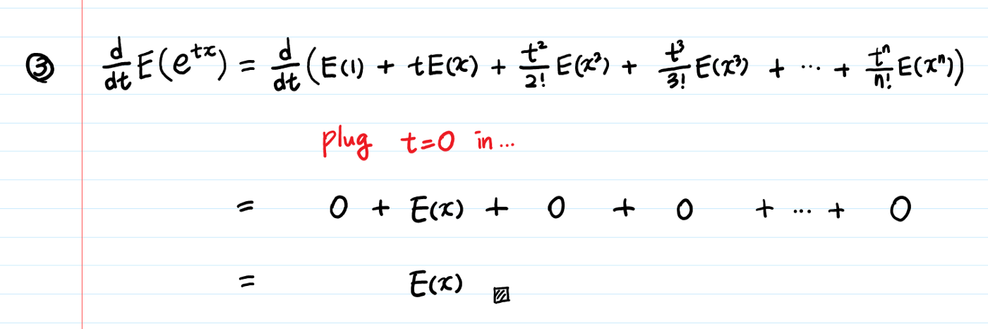
In this step, we take the first derivative of the equation only but similarly, we can prove that:

• If you take another derivative on equation-3 (therefore total twice), you will get E(X²).
• If you take the third derivative, you will get E(X³), and so on.

Note

When you try to deeply understand the concept behind the Moment-Generating Function, we couldn’t understand the role of t in the function, since t seemed like some arbitrary variable that we are not interested in. However, as you see, t is considered as a helper variable.

So, to be able to use calculus (derivatives) and make the terms (that we are not interested in) zero, we introduced the variable t.

Why do we need MGF?

We can calculate moments by using the definition of expected values but the question is that “Why do we need MGF exactly”?

For convenience,

To calculate the moments easily, we have to use the MGF. But

“Why is the calculation of moments using MGF easier than by using the definition of expected values”?

Let’s understand this concept with the help of the given below example that will cause a spark of joy in you — the clearest example where MGF is easier: 

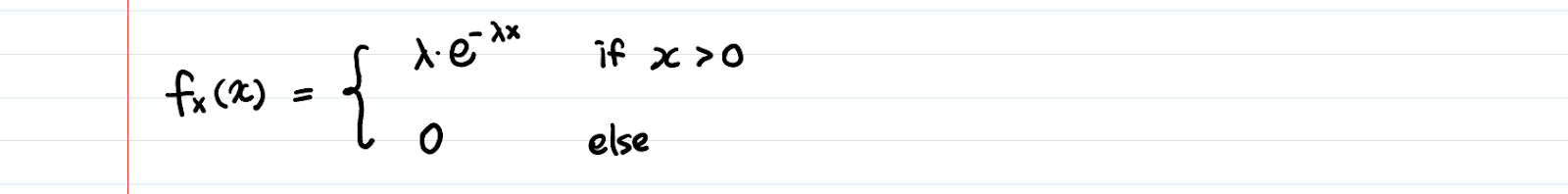
We will find the MGF of the exponential distribution.

Step-1: Firstly, we will start our discussion by writing the PDF of Exponential Distribution.

Step-2: With the help of pdf calculated in previous steps, now we determine the MGF of the exponential distribution.

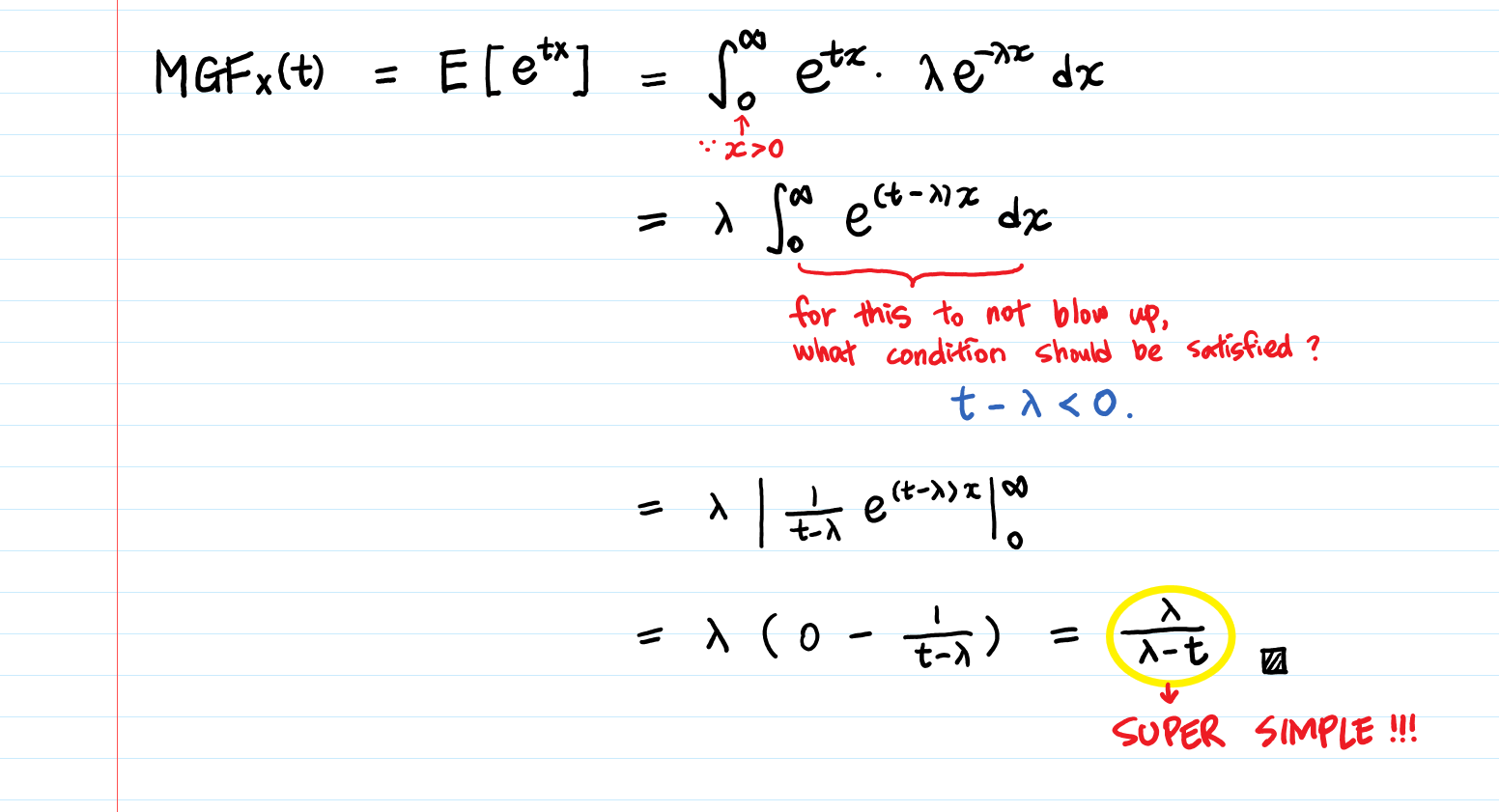
Now, for MGF to exist, the expected value E(e^tx) should exist.

Therefore, `t – λ < 0` becomes an important condition to meet, because if this condition doesn’t hold, then the integral won’t converge. This is known as the Divergence Test.

Once you have to find the MGF of the exponential distribution to be λ/(λ-t), then calculating moments becomes just a matter of taking derivatives, which is easier than the integrals to calculate the expected value directly.

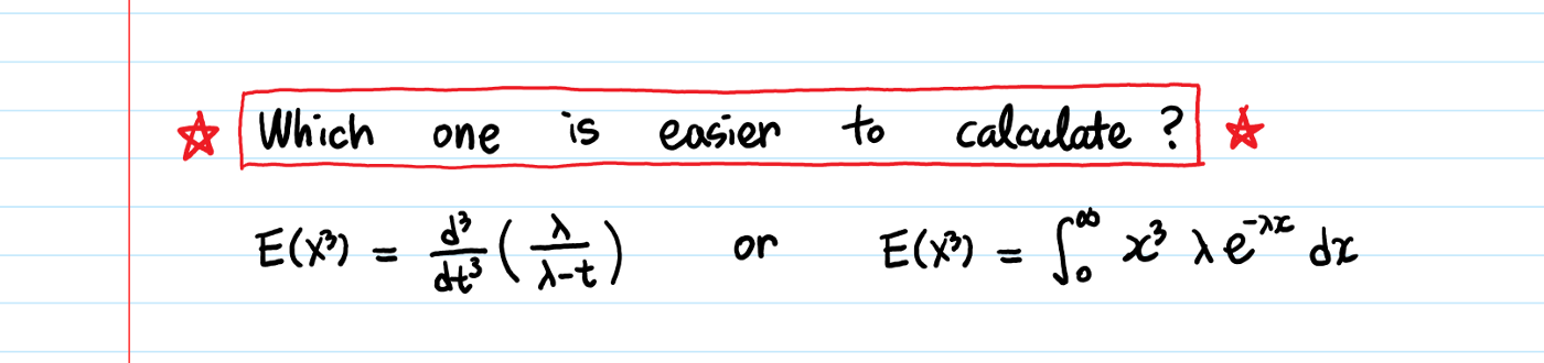
                                                     Image Source: Google Images

Therefore, with the help of MGF, it is possible to find moments by taking derivatives rather than doing integrals! So, this makes our life easier when dealing with statistical moments.

Important Results Related to MGF

Result-1: Sum of Independent Random Variables

Suppose X₁,…, X_n are n independent random variables, and the random variable Y is defined by

Y = X₁ + … + X_n.

Then, the moment-generating function of random variable Y is given as,

M_Y(t)=M_X1 (t)·…·M_Xn (t)

Result-2:

Suppose for two random variables X and Y we have M_X(t) = M_Y (t) < ∞ for all t in an interval, then X and Y have the same distribution.

Applications of MGF

1. Moments provide a way to specify a distribution:

We can completely specify the normal distribution by the first two moments, mean and variance. As we are going to know about multiple different moments of the distribution, then we will know more about that distribution.

For Example, If there is a person that you haven’t met, and you know about their height, weight, skin color, favorite hobby, etc., you still don’t necessarily fully know them but to getting more and more about them we can take the help of this.

2. Finding any n-th moment of a distribution:

We can get any n-th moment once you have MGF i.e, expected value exists. It encodes all the moments of a random variable into a single function from which we can be extracted again later.

3. Helps in determining Probability distribution uniquely:

Using MGF, we can uniquely determine a probability distribution. If two random variables have the same expression of MGF, then they must have the same probability distribution.

4. Risk Management in Finance: 

In this domain, one of the important characteristics of distribution is how heavy its tails are.

For Example: Consider the 2009 financial crisis, where we underestimated the chance of rare events. Risk managers often downplayed kurtosis, the fourth moment, in financial securities. Seemingly random distributions, masked by smooth risk curves, can hide unexpected peaks. Moment Generating Functions (MGF) help unveil these anomalies, aiding in bulge detection.

Problem Solving related to MGF

Problem Statement

Suppose that Y is a random variable with MGF H(t). Further, suppose that X is also a random variable with MGF M(t) which is given by, M(t) = 1/3 (2e^3t +1) H(t). Given that the mean of random variable Y is 10 and its variance is 12, then find the mean and variance of random variable X.

Solution:

Keep in mind all the results which we described above, we can say that

E(Y) = 10 ⇒ H'(0) =10,

E(Y²) – (E(Y))² = 12 ⇒ E(Y²) – 100 = 12 ⇒ E(Y²) = 112 ⇒ H”(0) = 112

M'(t) = 2e^3t H(t) + 1/3 ( 2e^3t +1 )H'(t)

M”(t) = 6e^3tH(t) + 4e^3tH'(t) + 1/3 ( 2e^3t +1 )H”(t)

Now, E(X) = M'(0) = 2H(0) + H'(0) = 2+10 =12

E(X²) = M”(0) = 6H(0) + 4H'(0) + H”(0) = 6 + 40 +112 = 158

Therefore, Var(X) = E(X²) – (E(X))² = 158 -144 = 14

So, the mean and variance of Random variable X are 12 and 14 respectively.

Conclusion

Moment-Generating Functions might sound fancy, but they’re a handy tool for data folks like us. We’ve seen how they help us find important stuff like averages and spreads in data. Remember, MGFs aren’t just theoretical—they’re real-world problem solvers. So, whether you’re a data scientist or just curious about numbers, keep MGFs in your toolkit—they’ll make your data adventures a whole lot easier! Happy crunching!

Frequently Asked Questions

This ends today’s discussion!