Covid-19 Tweets Analysis using NLP with Python
This article was published as a part of the Data Science Blogathon
Introduction
In this tutorial, I am going to discuss a practical guide of Natural Language Processing(NLP) using Python.
Before we move further, we will just take a look at the concept of Corona Virus namely CoVid-19.
CoVid-19: Coronavirus disease (CoVid-19) is an infectious disease that is caused by a newly discovered coronavirus. Most of the people who have been infected with the CoVid-19 virus will experience mild to adequate respiratory illness and some will recover without requiring any special treatment. Older or aged people and those with intrinsic medical problems like cardiovascular disease(heart diseases), diabetes, chronic respiratory disease, and cancer are more likely to create serious illnesses.

The COVID-19 virus can spread through droplets of saliva or release from the nose when an infected person coughs or sneezes.
Now we will see how to perform CoVid-19 tweets analysis. Let’s get started…
Dataset
Here I have used a dataset of coronavirus tweets NLP. You can find it out kaggle.com
Take a look at the description of the data:
The tweets have been taken from Twitter. Whatever the names and usernames have been given codes is just to avoid privacy concerns.
Columns:
1) Location- Location of user
2) Tweet At- Date of a tweet
3) Original Tweet- actual tweet text
4) Sentiment- sentiments(we can say emotions) like positive, negative, neutral, etc
Implementation
- Here we need to import the necessary libraries that be required for our model. In the above code, we have imported libraries such as pandas to deal with data frames/datasets, re for regular expression, nltk is a natural language tool kit and from that, we have imported module – stopwords which are nothing but ‘dictionary’. As shown below:
import pandas as pd
import numpy as np
import seaborn as sns
import matplotlib.pyplot as plt
import re
import nltk
nltk.download('stopwords')
from nltk.corpus import stopwords
[nltk_data] Downloading package stopwords to /root/nltk_data...
[nltk_data]   Unzipping corpora/stopwords.zip.
2) Here we have read the file named “Corona_NLP_train” in CSV(comma-separated value) format. And have checked for the top 5 values in the dataset using head()
data = pd.read_csv("Corona_NLP_train.csv",encoding='latin1')
df = pd.DataFrame(data)
df.head()
| UserName | ScreenName | Location | TweetAt | OriginalTweet | Sentiment | |
|---|---|---|---|---|---|---|
| 0 | 3799 | 48751 | London | 16-03-2020 | @MeNyrbie @Phil_Gahan @Chrisitv https://t.co/i… | Neutral |
| 1 | 3800 | 48752 | UK | 16-03-2020 | advice Talk to your neighbours family to excha… | Positive |
| 2 | 3801 | 48753 | Vagabonds | 16-03-2020 | Coronavirus Australia: Woolworths to give elde… | Positive |
| 3 | 3802 | 48754 | NaN | 16-03-2020 | My food stock is not the only one which is emp… | Positive |
| 4 | 3803 | 48755 | NaN | 16-03-2020 | Me, ready to go at supermarket during the #COV… | Extremely Negative |
3) Further, I have performed some data visualizations using matplotlib and seaborn libraries which are really the best visualization libraries in Python. I have plotted only one graph, you can plot more graphs to see how your data is!
plt.figure(figsize=(10,5))
sns.countplot(x='Sentiment', data=df, order=['Extremely Negative', 'Negative', 'Neutral', 'Positive', 'Extremely Positive'], )
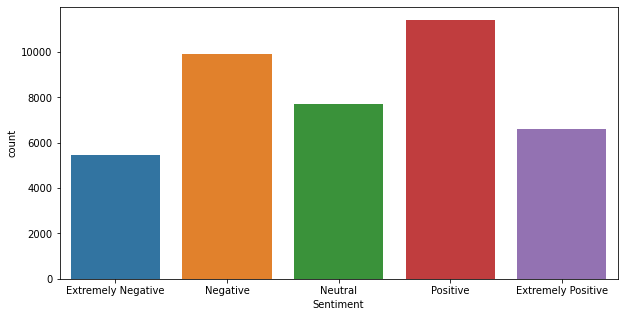
Graph of the Above code
4) In this step, we are able to see how the summary of our data like No. of columns with their data types.
df.info()
<class 'pandas.core.frame.DataFrame'> RangeIndex: 41157 entries, 0 to 41156 Data columns (total 6 columns): # Column Non-Null Count Dtype --- ------ -------------- ----- 0 UserName 41157 non-null int64 1 ScreenName 41157 non-null int64 2 Location 32567 non-null object 3 TweetAt 41157 non-null object 4 OriginalTweet 41157 non-null object 5 Sentiment 41157 non-null object dtypes: int64(2), object(4) memory usage: 1.9+ MB
5)Here we will perform a regular expression function to remove any symbols and special characters, etc to get pure data.
reg = re.compile("(@[A-Za-z0-9]+)|(#[A-Za-z0-9]+)|([^0-9A-Za-z t])|(w+://S+)")
tweet = []
for i in df["OriginalTweet"]:
  tweet.append(reg.sub(" ", i))
df = pd.concat([df, pd.DataFrame(tweet, columns=["CleanedTweet"])], axis=1, sort=False)
6) Now we can see cleaned data obtained from the above code.
df.head()
| UserName | ScreenName | Location | TweetAt | OriginalTweet | Sentiment | CleanedTweet | |
|---|---|---|---|---|---|---|---|
| 0 | 3799 | 48751 | London | 16-03-2020 | @MeNyrbie @Phil_Gahan @Chrisitv https://t.co/i… | Neutral | Gahan and and |
| 1 | 3800 | 48752 | UK | 16-03-2020 | advice Talk to your neighbours family to excha… | Positive | advice Talk to your neighbours family to excha… |
| 2 | 3801 | 48753 | Vagabonds | 16-03-2020 | Coronavirus Australia: Woolworths to give elde… | Positive | Coronavirus Australia Woolworths to give elde… |
| 3 | 3802 | 48754 | NaN | 16-03-2020 | My food stock is not the only one which is emp… | Positive | My food stock is not the only one which is emp… |
| 4 | 3803 | 48755 | NaN | 16-03-2020 | Me, ready to go at supermarket during the #COV… | Extremely Negative | Me ready to go at supermarket during the ou… |
7) now convert text into the matrix of tokens, we have to import the following library and perform code.
from sklearn.feature_extraction.text import TfidfVectorizer
stop_words = set(stopwords.words('english'))     # make a set of stopwords
vectoriser = TfidfVectorizer(stop_words=None)
8)LabelEncoder is used here for transforming categorical values into numerical values.
X_train = vectoriser.fit_transform(df["CleanedTweet"])
# Encoding the classes in numerical values
from sklearn.preprocessing import LabelEncoder
encoder = LabelEncoder()
y_train = encoder.fit_transform(df['Sentiment'])
from sklearn.naive_bayes import MultinomialNB
classifier = MultinomialNB()
classifier.fit(X_train, y_train)
9) Let’s do all operations for test data also.
# importing the Test dataset for prediction and testing purposes
test_data = pd.read_csv("Corona_NLP_test.csv",encoding='latin1')
test_df = pd.DataFrame(test_data)
test_df.head()
| UserName | ScreenName | Location | TweetAt | OriginalTweet | Sentiment | |
|---|---|---|---|---|---|---|
| 0 | 1 | 44953 | NYC | 02-03-2020 | TRENDING: New Yorkers encounter empty supermar… | Extremely Negative |
| 1 | 2 | 44954 | Seattle, WA | 02-03-2020 | When I couldn’t find hand sanitizer at Fred Me… | Positive |
| 2 | 3 | 44955 | NaN | 02-03-2020 | Find out how you can protect yourself and love… | Extremely Positive |
| 3 | 4 | 44956 | Chicagoland | 02-03-2020 | #Panic buying hits #NewYork City as anxious sh… | Negative |
| 4 | 5 | 44957 | Melbourne, Victoria | 03-03-2020 | #toiletpaper #dunnypaper #coronavirus #coronav… | Neutral |
10)Here we will perform a regular expression function to remove any symbols and special character, etc to get pure test data.
reg1 = re.compile("(@[A-Za-z0-9]+)|(#[A-Za-z0-9]+)|([^0-9A-Za-z t])|(w+://S+)")
tweet = []
for i in test_df["OriginalTweet"]:
tweet.append(reg1.sub(" ", i))
test_df = pd.concat([test_df, pd.DataFrame(tweet, columns=["CleanedTweet"])], axis=1, sort=False)
test_df.head()
| UserName | ScreenName | Location | TweetAt | OriginalTweet | Sentiment | CleanedTweet | |
|---|---|---|---|---|---|---|---|
| 0 | 1 | 44953 | NYC | 02-03-2020 | TRENDING: New Yorkers encounter empty supermar… | Extremely Negative | TRENDING New Yorkers encounter empty supermar… |
| 1 | 2 | 44954 | Seattle, WA | 02-03-2020 | When I couldn’t find hand sanitizer at Fred Me… | Positive | When I couldn t find hand sanitizer at Fred Me… |
| 2 | 3 | 44955 | NaN | 02-03-2020 | Find out how you can protect yourself and love… | Extremely Positive | Find out how you can protect yourself and love… |
| 3 | 4 | 44956 | Chicagoland | 02-03-2020 | #Panic buying hits #NewYork City as anxious sh… | Negative | buying hits City as anxious shoppers stock… |
| 4 | 5 | 44957 | Melbourne, Victoria | 03-03-2020 | #toiletpaper #dunnypaper #coronavirus #coronav… | Neutral | 19 One week everyone… |
11)By using vectorization, we have performed normalization of test data and stored it into x_test & y_test. We have also predicted actual and predicted values.
X_test = vectoriser.transform(test_df["CleanedTweet"])
y_test = encoder.transform(test_df["Sentiment"])
# Prediction
y_pred = classifier.predict(X_test)
pred_df = pd.DataFrame({'Actual': y_test, 'Predicted': y_pred})
pred_df.head()
| Actual | Predicted | |
|---|---|---|
| 0 | 0 | 2 |
| 1 | 4 | 4 |
| 2 | 1 | 4 |
| 3 | 2 | 2 |
| 4 | 3 | 2 |
12)So, at last, we have performed the accuracy of our model in the form of an AUC curve plotted using the matplotlib library.
from sklearn import metrics
# Generate the roc curve using scikit-learn.
fpr, tpr, thresholds = metrics.roc_curve(y_test, y_pred, pos_label=1)
plt.plot(fpr, tpr)
plt.xlabel('False positive rate')
plt.ylabel('True positive rate')
plt.title('ROC curve')
plt.show()
# Measure the area under the curve. The closer to 1, the "better" the predictions.
print("AUC of the predictions: {0}".format(metrics.auc(fpr, tpr)))
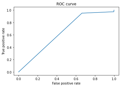
AUC of the predictions: 0.6389011382417605
Here we got a score of AUC – 0.64 for the classifier (Naive Byes), we can say that the classifier (Naive Bayes) is not that so good but can acceptable. Since the more nearer to 1 AUC score, the classifier will be better.
In the same way, we can perform any sentimental analysis of “tweets”.
Conclusion
I hope you liked my article. Please do share with your friends, colleagues. Thank You!
The media shown in this article are not owned by Analytics Vidhya and are used at the Author’s discretion.
I am data science enthusiastic, tech savvy and traveller.


