Crowd Counting using Deep Learning
This article was published as a part of the Data Science Blogathon
Introduction
Before we start with Crowd Counting, let’s get familiar with counting objects in images. It is one of the fundamental tasks in computer vision. The goal of Object Counting is to count the number of object instances in a single image or video sequence. It has many real-world applications such as surveillance, microbiology, crowdedness estimation, product counting, and traffic flow monitoring.
Types of object counting techniques
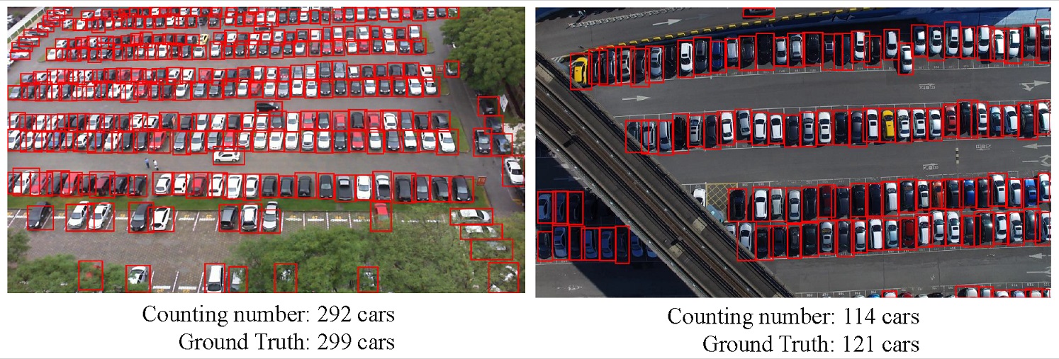
1. Detection-based Object Counting – Here, we use a moving window-like detector to identify the target objects in an image and count how many there are. The methods used for detection require well-trained classifiers that can extract low-level features. Although these methods work well for detecting faces, they do not perform well on crowded images of people/objects as most of the target objects are not clearly visible.
An implementation of detection-based object counting can be done using any state-of-the-art object detection methods like Faster RCNN or Yolo where the model detects the target objects in the images. We can return the count of the detected objects (the bounding boxes) to obtain the count.
2. Regression-based Object Counting – We build an end-to-end regression method using CNNs. This takes the entire image as input and directly generates the crowd/object count. CNNs work really well with regression or classification tasks. The regression-based method directly maps the number of objects predicted based on features extracted from cropped image patches to the ground truth count.
An implementation of regression-based object counting has been seen in Kaggle’s NOAA fisheries steller sea lion population count competition where the winner had used VGG-16 as the feature extractor and created a fully connected architecture with the last layer being a regression layer (linear output).
Now since we have discussed some of the basics of object counting, let us start Crowd Counting!
Crowd Counting
Crowd Counting is a technique to count or estimate the number of people in an image. Accurately estimating the number of people/objects in a single image is a challenging yet meaningful task and has been applied in many applications such as urban planning and public safety. Crowd counting is particularly prominent in the various object counting tasks due to its specific significance to social security and development.
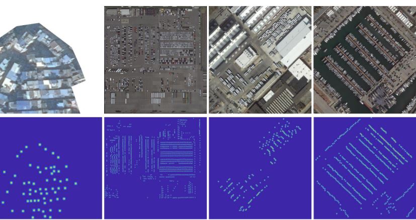
Before we proceed further, look at various crowd counting datasets to know how the crowd images actually look like!
Types of approaches for crowd counting technique –
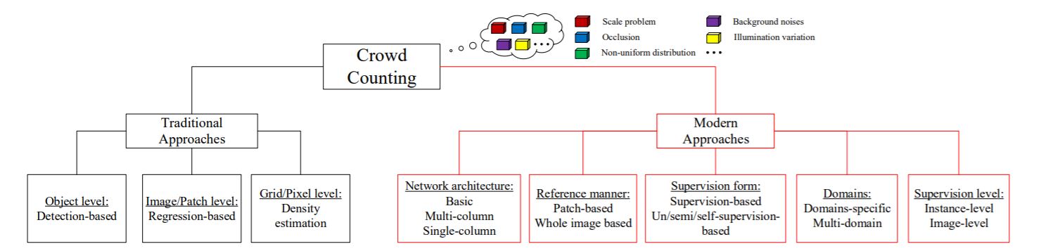
Problem
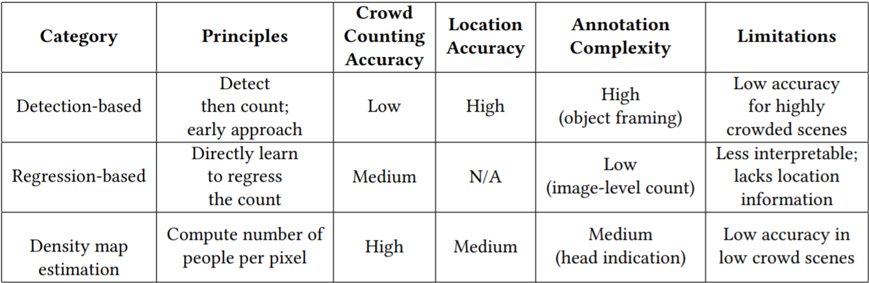
- Early works on crowd counting use detection-based approaches(we have already discussed the basics of the detection-based approach). These approaches usually apply a person head detector via a moving window on an image. Recently many extraordinary object detectors such as R-CNN, YOLO, and SSD have been presented, which may perform dramatic detection accuracy in sparse scenes. However, they will present unsatisfactory results when encountered the situation of occlusion and background clutter in extremely dense crowds.
- To reduce the above problems, some works introduce regression-based approaches which directly learn the mapping from an image patch to the count. They usually first extract global features (texture, gradient, edge features), or local features (SIFT, LBP, HOG, GLCM). Then some regression techniques such as linear regression are used to learn a mapping function to the crowd counting. These methods are successful in dealing with the problems of occlusion and background clutter, but they always
ignore spatial information.
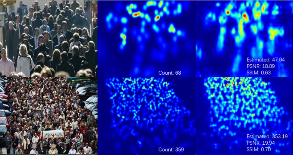
Density Estimation based method
is a method to solve this problem by learning a linear mapping between features in the local region and its object density maps. It integrates the information of saliency during the learning process. Since the ideal linear mapping is hard to obtain, we can use random forest regression to learn a non-linear mapping instead of the linear one.
The latest works have used CNN-based approaches to predict the density map because of its success in classification and recognition. In the rest of the blog, we will some of the modern density map-based approach methods mainly CNN-based for crowd counting. By the end of the blog, you’ll have an intuition of how crowd counting techniques work and how to implement them!
Ground truth generation –
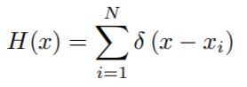
- Assuming that there is an object instance (head of a person in our case) at pixel xi, it can be represented by a delta function δ(x − xi). Therefore, for an image with N annotations, it can be represented by the above equation
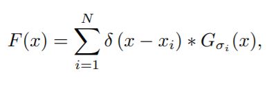
where σi represents the standard deviation
- To generate the density map F, we convolute H(x) with a Gaussian kernel, which can be defined by the above equation.
1. MCNN – Multi-column CNN for density map estimation.
- The images of the crowd usually contain heads of very different sizes, hence filters with receptive fields of the same size are unlikely to capture characteristics of crowd density at different scales. Therefore, it is more natural to use filters with different sizes of local receptive fields to learn the map from the raw pixels to the density maps. In MCNN, for each column, we use filters of different sizes to model the density maps corresponding to heads of different scales. For instance, filters with larger receptive fields are more useful for modeling the density maps corresponding to larger heads.
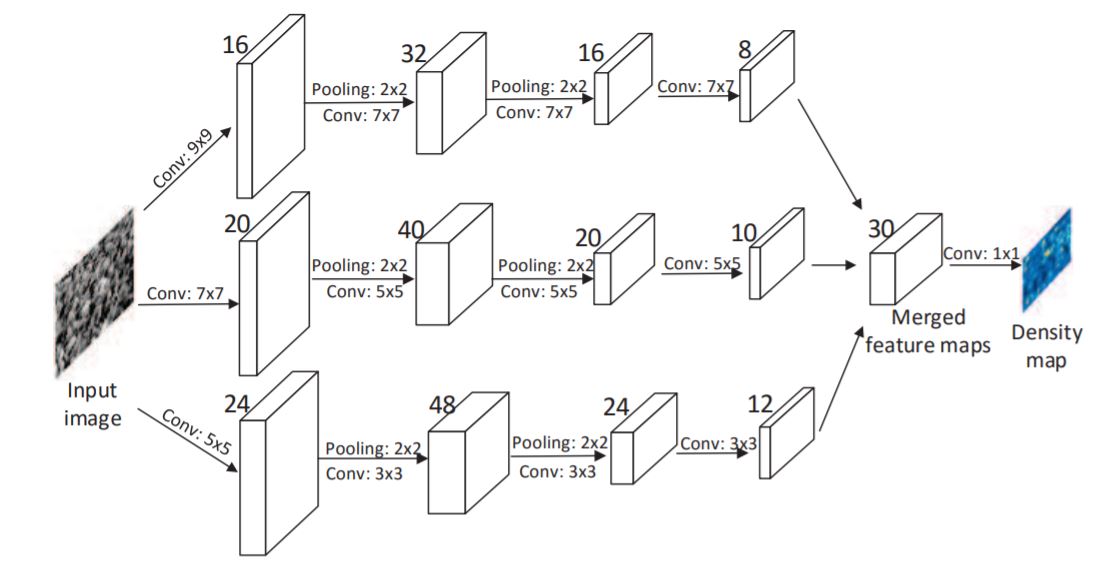
- It contains three parallel CNNs whose filters are with local receptive fields of different sizes. For simplification, we use the same network structures for all columns (i.e., conv–pooling–conv–pooling) except for the sizes and numbers of filters. Max pooling is applied for each 2×2 region, and Rectified linear unit (ReLU) is adopted as the activation function because of its good performance for CNNs . To reduce the computational complexity (the number of parameters to be optimized), we use fewer filters for CNNs with larger filters. We stack the output feature maps of all CNNs and map them to a density map. To map the features maps to the density map, we adopt filters whose sizes are 1 × 1.
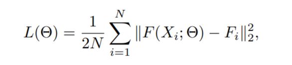
- Then Euclidean distance is used to measure the difference between the estimated density map and ground truth. The loss is defined as –
Refer to the papers and code to learn more about MCNN. The method was proposed on the Shanghaitech crowd dataset.
2. CSRNet – Dilated Convolutional Neural Networks for Understanding the Highly Congested Scenes
- The proposed CSRNet is composed of two major components: a convolutional neural network (CNN) as the front-end for 2D feature extraction and a dilated CNN for the back-end, which uses dilated kernels to deliver larger reception fields and to replace pooling operations. CSRNet is an easy-trained model because of its pure convolutional structure.
- They chose VGG16 as the front-end of CSRNet because of its strong transfer-learning ability and its flexible architecture for easily concatenating the back-end for density map generation. In these cases, the VGG-16 performs as an ancillary without significantly boosting the final accuracy. In the research paper, they first remove the classification part of VGG16 (fully connected layers) and build the proposed CSRNet with convolutional layers in VGG-16.
- The output size of this front-end network is 1/8 of the original input size. If we continue to stack more convolutional layers and pooling layers (basic components in VGG-16), output size would be further shrunken, and it is hard to generate high-quality density maps. Therefore they deployed dilated convolutional layers as the back-end.
-
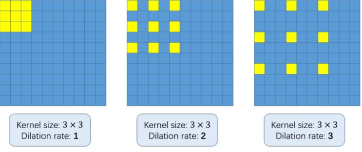
- In dilated convolution, a small-size kernel with a k × k filter is enlarged to k + (k − 1)(r − 1) with dilated stride r. Thus it allows flexible aggregation of the multi-scale contextual information while keeping the same resolution. Dilated convolution is applied to keep the output resolutions high and it avoids the need for upsampling. Most importantly, the output from dilated convolution contains more detailed information (referring to the portions we zoom in on). Read this to understand more about dilated convolution.
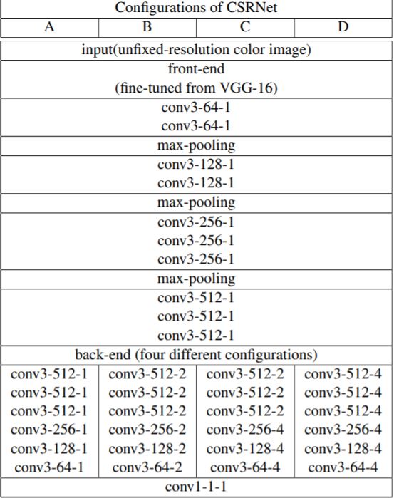
- Configuration – They kept the first ten layers of VGG-16 with only three pooling layers instead of five to suppress the detrimental effects on output accuracy caused by the pooling operation. Since the output (density maps) of CSRNet is smaller (1/8 of input size), we choose bilinear interpolation with the factor of 8 for scaling and make sure the output shares the same resolution as the input image.
- Refer to the papers and code to learn more about CSRNet. The method gave state-of-the-art results on various crowd counting datasets.
Now we have come to the end of the blog! Refer to this to know more about crowd counting methods. Do give your feedback about the blog in the comments. Happy Learning 🙂
About the author
I am Yash Khandelwal, pursuing MSc in Mathematics and Computing from Birla Institute of Technology, Ranchi. I am a Data Science and Machine Learning enthusiast.
Feel free to connect! https://www.linkedin.com/in/yash-khandelwal-a40484bb/
Github – https://github.com/YashK07
The media shown in this article are not owned by Analytics Vidhya and are used at the Author’s discretion.


Thanks for neat explanation. It’s so helpful for me to know where to go!