Decide Best Learning Rate with LearningRateScheduler in Tensorflow
This article was published as a part of the Data Science Blogathon
Validation for your correct decisions feels so much better and relaxing
Imagine you are doing a task for the first time and an expert suddenly comments that you are doing a good job, keep it up. I won’t say anything about you but for me, that comment is more than enough to boost my motivation towards completing the task and feeling relatively less anxious for the actions.
Now, coming back to Machine learning (Deep learning to be precise), if something tells you during the task that whatever you are doing with your neural networks, I am sure your learning rate seems fine. Wouldn’t that be great! Wouldn’t you feel less uncertain about your learning rate as one of the hyperparameter? Well, after discovering LearningRateScheduler I certainly felt great.
Learning Rate: In deep learning terminology, the learning rate is the coefficient of the gradient calculated which is reduced from your parameters during backpropagation to tune them in accordance to minimize the cost function. In layman terms, It signifies how much change do you want your parameters to go through after each training cycle (forward propagation and backward propagation).
Today, during the journey to discover and see LearningRateScheduler in action, we will be working on mathematically generated synthetic time series data. I have already written a dedicated article for this dataset and time-series data in general which will help you get started towards deep learning on time series data.
What is LearningRateScheduler ?
LearningRateScheduler is one of the callbacks in Keras API (Tensorflow). Callbacks are those utilities that are called during the training at certain points depending on each particular callback. Whenever we are training our neural network, these callbacks are called in between the training to perform their respective tasks. For example in our case, At the beginning of every epoch, the LearningRateScheduler callback gets the updated learning rate value from the schedule function that we define ahead of time before training, with the current epoch and current learning rate, and applies the updated learning rate on the optimizer.
Let us look at it in action while training a simple neural network for our synthetic time series data.
1. Generating the Synthetic Time-Series
First of all, import all the necessary libraries:
import tensorflow as tf
import numpy as np
import matplotlib.pyplot as plt
Second of all, create a helper function to plot time series data to avoid redundant code:
def plot_series(time,series, format = '-', start =0, end = None):
    plt.plot(time[start:end], series[start:end], format)
    plt.xlabel("Time")
    plt.ylabel("Series")
    plt.grid(True)
Third of all, let’s finally define those function that will help us generate our synthetic time series data. For understanding more about how they are created and what they represent, I highly recommend you checking out this post on Deep Dive into Time Series Data. Here are those functions:
def trend(time, slope=0):
    return time*slope
def seasonal_pattern(season_time):
    return np.where(season_time<0.4,
                  np.cos(season_time * 2*np.pi),
                  1/np.exp(3*season_time))
def seasonality(time, period, amplitude=1, phase = 0):
    season_time = ((time+phase)%period)/period
    return amplitude*seasonal_pattern(season_time)
def noise(time, noise_level = 1, seed=None):
    rnd = np.random.RandomState(seed)
    return rnd.randn(len(time))*noise_level
Connecting all these features with the logic to create a time series data (don’t worry about the math behind it, It is not in the scope of this article).
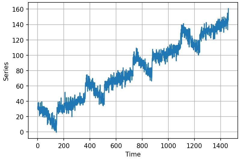
time = np.arange(4*365+1,dtype='float32')
baseline = 10
series = trend(time, slope=0.1)
amplitude = 20
slope = 0.09
noise_level = 5
series = baseline+ trend(time,slope) + seasonality(time, period=365, amplitude=amplitude)
series+=noise(time, noise_level, seed = 42)
Look at the time series using our defined helper function ‘plot_series()’
plot_series(time,series)
2. Preparing the Dataset for Training and Testing
First, we will divide the time series into training and testing data. Remember, In time-series data, sequences of the values are extremely important because they are what our features and representation to predict values would be.
Secondly, after the train-test split, we will use Tensorflow Dataset API to create a windowed dataset, which is what we do pretty much every time when working with time series and non-sequence specific neural networks like (RNNs or LSTMs). For more detail on the topic of the windowed dataset check out the Deep Dive into Time Series Data.
## Train-Test Split
split_time = 1000
train_series = series[:split_time]
train_time = time[:split_time]
valid_series = series[split_time:]
valid_time = time[split_time:]
#Tensorflow Dataset API for windowed dataset
def windowed_dataset(series, window_size, batch_size, shuffle_batch_size):
    dataset = tf.data.Dataset.from_tensor_slices(series)
    dataset = dataset.window(window_size+1, 1, drop_remainder = True)
    dataset = dataset.flat_map(lambda window: window.batch(window_size+1))
    dataset = dataset.shuffle(shuffle_batch_size).map(lambda window: (window[:-1], window[-1:]))
    dataset = dataset.batch(batch_size).prefetch(1)
    return dataset
# Calling the Function to get the data in 'dataset' variable
window_size = 20
batch_size = 32
shuffle_batch_size = 1000
dataset = windowed_dataset(train_series, window_size, batch_size, shuffle_batch_size)
3. Neural Network and LearningRateScheduler
model = tf.keras.models.Sequential([
                                    tf.keras.layers.Dense(10, activation='relu', input_shape = [window_size]),
                                    tf.keras.layers.Dense(10, activation='relu'),
                                    tf.keras.layers.Dense(1)
])
lr_schedule = tf.keras.callbacks.LearningRateScheduler(
    lambda epoch: 1e-8 * 10**(epoch/20)
)
model.compile(loss= 'mse', optimizer=tf.keras.optimizers.SGD(1e-8, momentum=0.9))
history = model.fit(dataset, epochs= 100, callbacks=[lr_schedule], verbose=0)
The first section of the code is for creating a Neural Network with 3 Dense Fully connected layers having ‘relu’ activation in the first 2 of them.
The second section of the code is what I mentioned earlier about the scheduler function which gets called during training by LearningRateScheduler callback to change its learning rate. Here this function is changing the learning rate from 1e-8 to 1e-3.
The third section is the simple compilation of the network with model.compile, while having an additional parameter ‘callbacks‘ in the model.fit function where we need to provide an iterator with callbacks listed which will be called during training i.e., lr_schedule.
NOTE: This model.fit is not our actual training of the model on the given dataset so don’t worry after seeing an unusual change in loss values, it is merely used to experiment with different learning rates that are automatically changing during training. The one with the least noise in the loss function would be our ideal learning rate.
After your model is done with fitting, certain values are stored in this history variable regarding our current training process. Let’s visualize the loss curvature to find the lowest smoother values in the curve with the x-axis in the logrithimic range (because the change in learning rate is far exponential to change in loss).
lrs = 1e-8 * (10**(np.arange(100)/20))
plt.semilogx(lrs, history.history['loss'])
plt.axis([1e-8, 1e-3, 0 , 300])
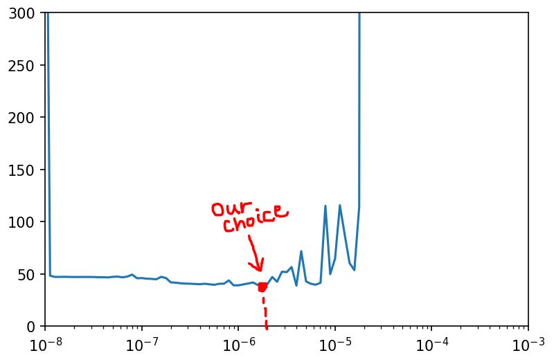
It is a visual choice to select whichever value you find the lowest with smoothness maintained. In my case, I took the point mentioned in figure (3e-6).
After you decide your learning rate, now is the time to get your hands dirty with the actual training of the model on the given dataset.
4. Training and Testing the Model
Now notice, we won’t be using lr_schedule as a callback because now there is no need to change the learning rate during training as we have already got an almost optimum one with experimentation.
model = tf.keras.models.Sequential([
tf.keras.layers.Dense(10, activation='relu', input_shape = [window_size]),
tf.keras.layers.Dense(10, activation='relu'),
tf.keras.layers.Dense(1)
])
model.compile(loss= 'mse', optimizer=tf.keras.optimizers.SGD(3e-6, momentum=0.9)) ## We picked 3e-6 from the graph
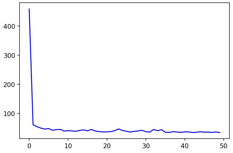
history = model.fit(dataset, epochs= 50, verbose=0)
Just Observe the power that we gave to our network by selecting a great learning rate after this training is completed, how much faster your model converged!. In 10 epochs you almost got the optimum loss, and further, along the 10 epochs, the line looks almost flat.
loss = history.history['loss']
epochs = range(len(loss))
plt.figure(dpi = 150)
plt.plot(epochs, loss, 'b', label="training_loss")
plt.show()
Testing/ Forecasting the Model:
forecast = []
for time in range(len(series)-window_size):
    forecast.append(model.predict(series[time:time+window_size][np.newaxis]))
forecast = forecast[split_time-window_size:]
results = np.array(forecast)[: , 0,0]
The way we test Time Series windowed dataset is a little different to what you might be used to. To read more on this, check out the above-mentioned article: Deep Dive into Time Series Data.
Visualizing the Forecasting:
plt.figure(figsize=(10,6))
plot_series(valid_time, valid_series)
plot_series(valid_time, results)
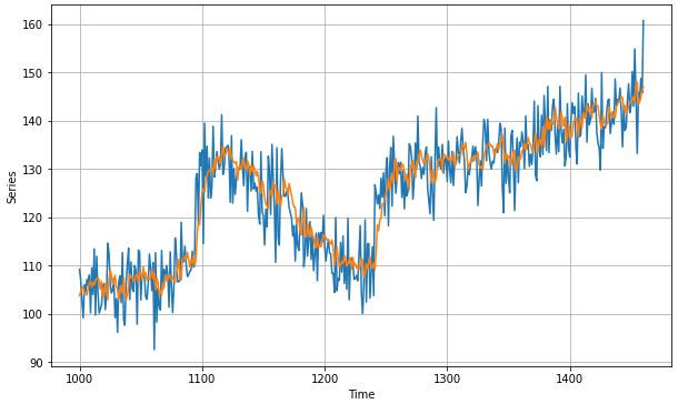
As a metric, we can look at Mean Absolute Loss to see how well did our model performed:
tf.keras.metrics.mean_absolute_error(valid_series, results).numpy()
MAE: 4.4020 (which is significantly good for such a simple model)
That’s it from this article, I hope you loved that such powerful and easy to do things exist for us to make better A.I. models. I know, I adore it very much.
Gargeya Sharma
B.Tech Computer Science 4th year
Specialized in Data Science and Deep Learning
Data Scientist Intern at Upswing Cognitive Hospitality Solutions
For more info check out my Github Home Page
Photo by Jake Givens on Unsplash


