Defining, Analysing, and Implementing Imputation Techniques
This article was published as a part of the Data Science Blogathon
What is Data Imputation?
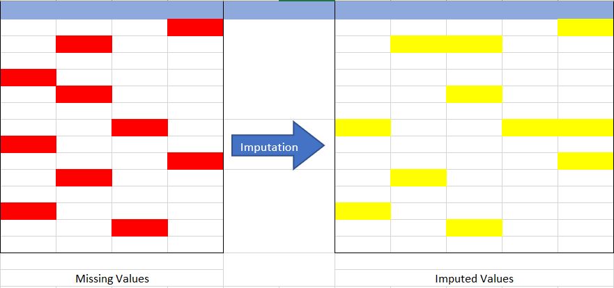
Imputation is a technique used for replacing the missing data with some substitute value to retain most of the data/information of the dataset. These techniques are used because removing the data from the dataset every time is not feasible and can lead to a reduction in the size of the dataset to a large extend, which not only raises concerns for biasing the dataset but also leads to incorrect analysis.
Source: created by Author
Not Sure What is Missing Data ? How it occurs? And its type? Have a look HERE to know more about it.
Let’s understand the concept of Imputation from the above Fig {Fig 1}. In the above image, I have tried to represent the Missing data on the left table(marked in Red) and by using the Imputation techniques we have filled the missing dataset in the right table(marked in Yellow), without reducing the actual size of the dataset. If we notice here we have increased the column size, which is possible in Imputation(Adding “Missing” category imputation).
Why Data Imputation is Important?
So, after knowing the definition of Imputation, the next question is Why should we use it, and what would happen if I don’t use it?
Here we go with the answers to the above questions
We use imputation because Missing data can cause the below issues: –
- Incompatible with most of the Python libraries used in Machine Learning:- Yes, you read it right. While using the libraries for ML(the most common is skLearn), they don’t have a provision to automatically handle these missing data and can lead to errors.
- Distortion in Dataset:- A huge amount of missing data can cause distortions in the variable distribution i.e it can increase or decrease the value of a particular category in the dataset.
- Affects the Final Model:- the missing data can cause a bias in the dataset and can lead to a faulty analysis by the model.
Another and the most important reason is “We want to restore the complete dataset”. This is mostly in the case when we do not want to lose any(more of) data from our dataset as all of it is important, & secondly, dataset size is not very big, and removing some part of it can have a significant impact on the final model.
Great..!! we got some basic concepts of Missing data and Imputation. Now, let’s have a look at the different techniques of Imputation and compare them. But before we jump to it, we have to know the types of data in our dataset.
Sounds strange..!!! Don’t worry… Most data is of 4 types:- Numeric, Categorical, Date-time & Mixed. These names are quite self-explanatory so not going much in-depth and describing them.
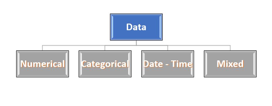
Fig 2:- Types of Data
Source: created by Author
Data Imputation Techniques
Moving on to the main highlight of this article – techniques used in data imputation.
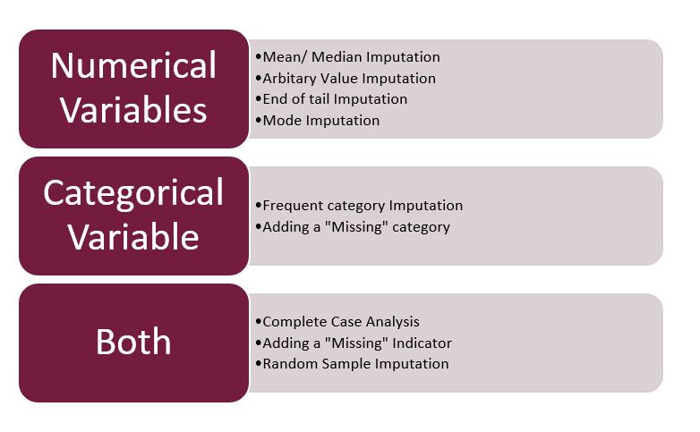
Fig 3:- Imputation Techniques
Source: created by Author
Note:- I will be focusing only on Mixed, Numerical and Categorical Imputation here. Date-Time will be part of next article.
1. Complete Case Analysis(CCA):-
This is a quite straightforward method of handling the Missing Data, which directly removes the rows that have missing data i.e. we consider only those rows where we have complete data i.e. data is not missing. This method is also popularly known as “Listwise deletion”.
- Assumptions:-
- Data is Missing At Random(MAR).
- Missing data is completely removed from the table.
- Advantages:-
- Easy to implement.
- No Data manipulation required.
- Limitations:-
- Deleted data can be informative.
- Can lead to the deletion of a large part of the data.
- Can create a bias in the dataset, if a large amount of a particular type of variable is deleted from it.
- The production model will not know what to do with Missing data.
- When to Use:-
- Data is MAR(Missing At Random).
- Good for Mixed, Numerical, and Categorical data.
- Missing data is not more than 5% – 6% of the dataset.
- Data doesn’t contain much information and will not bias the dataset.
- Code:-
## To check the shape of original dataset
train_df.shape
## Output (614 rows & 13 columns)
(614,13)
## Finding the columns that have Null Values(Missing Data)
## We are using a for loop for all the columns present in dataset with average null values greater than 0
na_variables = [ var for var in train_df.columns if train_df[var].isnull().mean() > 0 ]
## Output of column names with null values
['Gender','Married','Dependents','Self_Employed','LoanAmount','Loan_Amount_Term','Credit_History']
## We can also see the mean Null values present in these columns {Shown in image below}
data_na = trainf_df[na_variables].isnull().mean()
## Implementing the CCA techniques to remove Missing Data
data_cca = train_df(axis=0)  ### axis=0 is used for specifying rows
## Verifying the final shape of the remaining dataset
data_cca.shape
## Output (480 rows & 13 Columns)
(480,13)
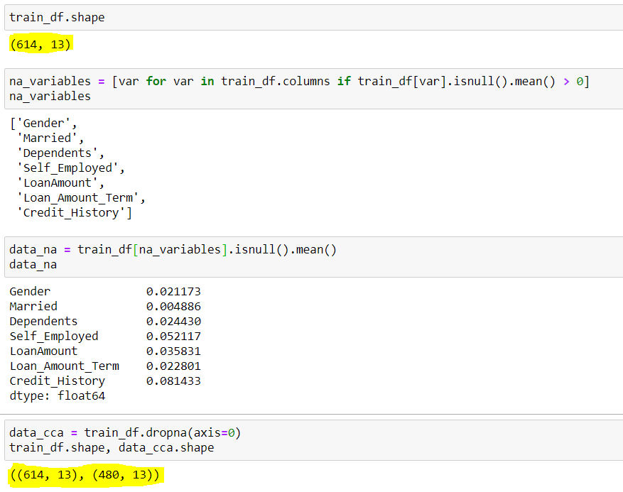
Fig 3:- CCA
Source: Created by Author
Here we can see, dataset had initially 614 rows and 13 columns, out of which 7 rows had missing data(na_variables), their mean missing rows are shown by data_na. We notice that apart from <Credit_History> & <Self_Employed> all have mean less than 5%. So as per the CCA, we dropped the rows with missing data which resulted in a dataset with only 480 rows. Around 20% of the data reduction can be seen here, which can cause many issues going ahead.
2. Arbitrary Value Imputation
This is an important technique used in Imputation as it can handle both the Numerical and Categorical variables. This technique states that we group the missing values in a column and assign them to a new value that is far away from the range of that column. Mostly we use values like 99999999 or -9999999 or “Missing” or “Not defined” for numerical & categorical variables.
- Assumptions:-
- Data is not Missing At Random.
- The missing data is imputed with an arbitrary value that is not part of the dataset or Mean/Median/Mode of data.
- Advantages:-
- Easy to implement.
- We can use it in production.
- It retains the importance of “missing values” if it exists.
- Disadvantages:-
- Can distort original variable distribution.
- Arbitrary values can create outliers.
- Extra caution required in selecting the Arbitrary value.
- When to Use:-
- When data is not MAR(Missing At Random).
- Suitable for All.
- Code:-
## Finding the columns that have Null Values(Missing Data)
## We are using a for loop for all the columns present in dataset with average null values greater than 0
na_variables = [ var for var in train_df.columns if train_df[var].isnull().mean() > 0 ]
## Output of column names with null values
['Gender','Married','Dependents','Self_Employed','LoanAmount','Loan_Amount_Term','Credit_History']
## Use Gender column to find the unique values in the column
train_df['Gender'].unique()
## Output
array(['Male','Female',nan])
## Here nan represent Missing Data
## Using Arbitary Imputation technique, we will Impute missing Gender with "Missing"  {You can use any other value also}
arb_impute = train_df['Gender'].fillna('Missing')
arb.impute.unique()
## Output
array(['Male','Female','Missing'])
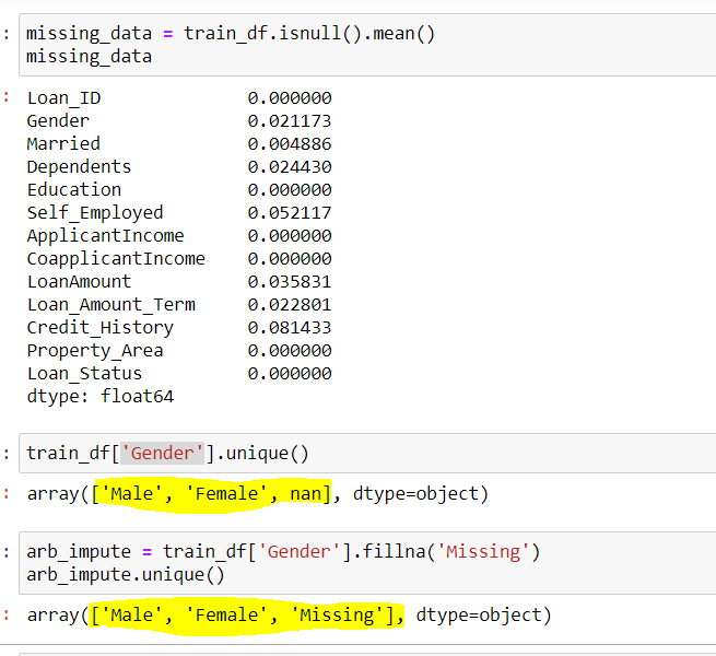
Fig 4:- Arbitrary Imputation
Source: created by Author
We can see here column Gender had 2 Unique values {‘Male’,’Female’} and few missing values {nan}. By using the Arbitrary Imputation we filled the {nan} values in this column with {missing} thus, making 3 unique values for the variable ‘Gender’.
3. Frequent Category Imputation
This technique says to replace the missing value with the variable with the highest frequency or in simple words replacing the values with the Mode of that column. This technique is also referred to as Mode Imputation.
- Assumptions:-
- Data is missing at random.
- There is a high probability that the missing data looks like the majority of the data.
- Advantages:-
- Implementation is easy.
- We can obtain a complete dataset in very little time.
- We can use this technique in the production model.
- Disadvantages:-
- The higher the percentage of missing values, the higher will be the distortion.
- May lead to over-representation of a particular category.
- Can distort original variable distribution.
- When to Use:-
- Data is Missing at Random(MAR)
- Missing data is not more than 5% – 6% of the dataset.
- Code:-
## finding the count of unique values in Gender
train_df['Gender'].groupby(train_df['Gender']).count()
## Output (489 Male & 112 Female)
Male 489
Female 112
## Male has higgest frequency. We can also do it by checking the mode
train_df['Gender'].mode()
## Output
Male
## Using Frequent Category Imputer
frq_impute = train_df['Gender'].fillna('Male')
frq_impute.unique()
## Output
array(['Male','Female'])
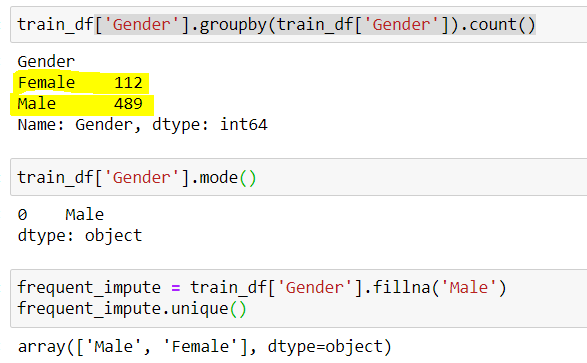
Fig 4:- Frequent Category Imputer
Source: created by Author
Here we noticed “Male” was the most frequent category thus, we used it to replace the missing data. Now we are left with only 2 categories i.e. Male & Female.
Thus, we can see every technique has its Advantages and Disadvantages, and it depends upon the dataset and the situation for which different techniques we are going to use.
The media shown in this article are not owned by Analytics Vidhya and are used at the Author’s discretion.


The assumption under which the listwise deletion is recommended is not MAR as you wrote. But it is rather MCAR (missing completely a random) which should not be confused with missing at random MAR.