Face Detection and Recognition capable of beating humans using FaceNet

This article was published as a part of the Data Science Blogathon

Creating face recognition is considered to be a very easy task in the field of computer vision, but it is extremely tough to have a pipeline that can predict faces with complex backgrounds when you have multiple faces, different lighting conditions, and different scales of images. This blog will describe how we made a model that can outperform humans in some cases. Our dataset consists of 3 classes (I can’t share the data due to confidentiality issues, but I’ll show you how it looks). Class 1 is Jesse Eisenberg(Actor), class 2 is Mila Kunis (Pop Star), and class 0, any person. Here’s how our train (80 images) and test data (1800+ images) looked like.

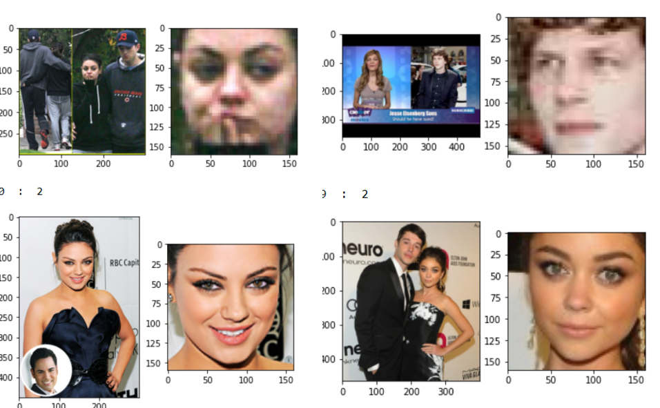
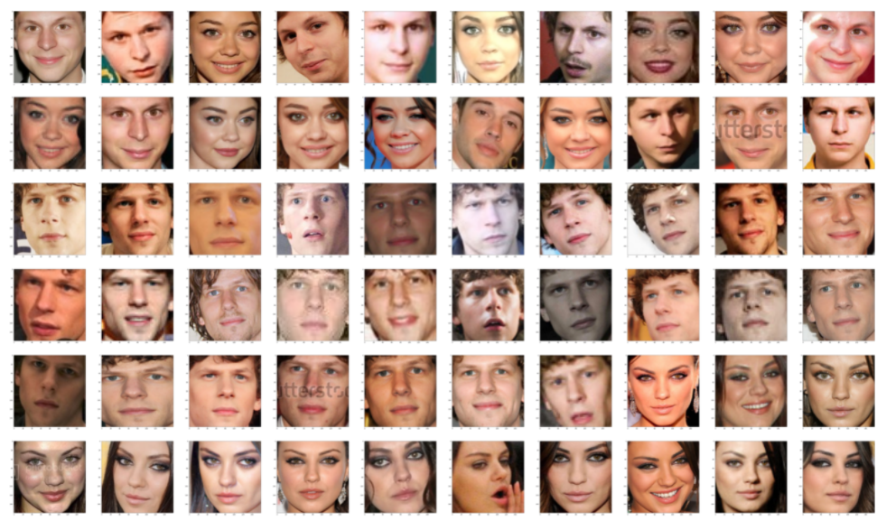
This is our test data and the extracted faces from those images, this data has extreme complexity due to multiple faces, complex backgrounds, and a lot of pixelated images. On the other hand, our train data is extremely clean shown in the below image. We have quite a lot of differences in the train and test data distribution. We need a technique that can generalize well irrespective of the number of samples it needs and how different the train and test data are.

The technique we are going to use for this task is, firstly, generate the face embedding from a deep learning model and then apply a simple classifier.

Using FACENET

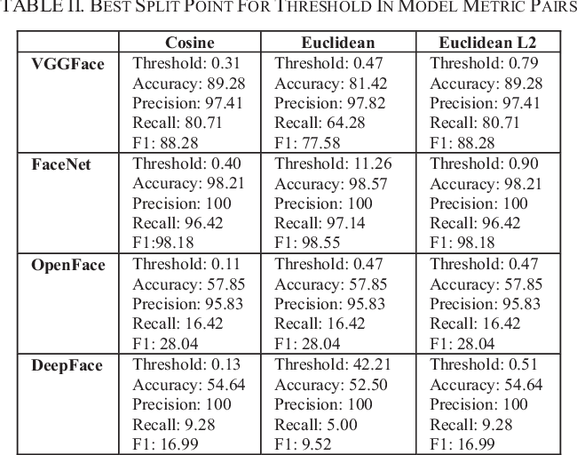
To really push the limits of face detection we will look at some state-of-the-art methods. Modern-day face extraction techniques have made use of Deep Convolution Networks. As we all know that features created by modern deep learning frameworks are really better than most handcrafted features. We checked 4 deep learning models namely, FaceNet (Google), DeepFace (Facebook), VGGFace (Oxford), and OpenFace (CMU). Out of these 4 models FaceNet was giving us the best result. In general, FaceNet gives better results than all the other 3 models.

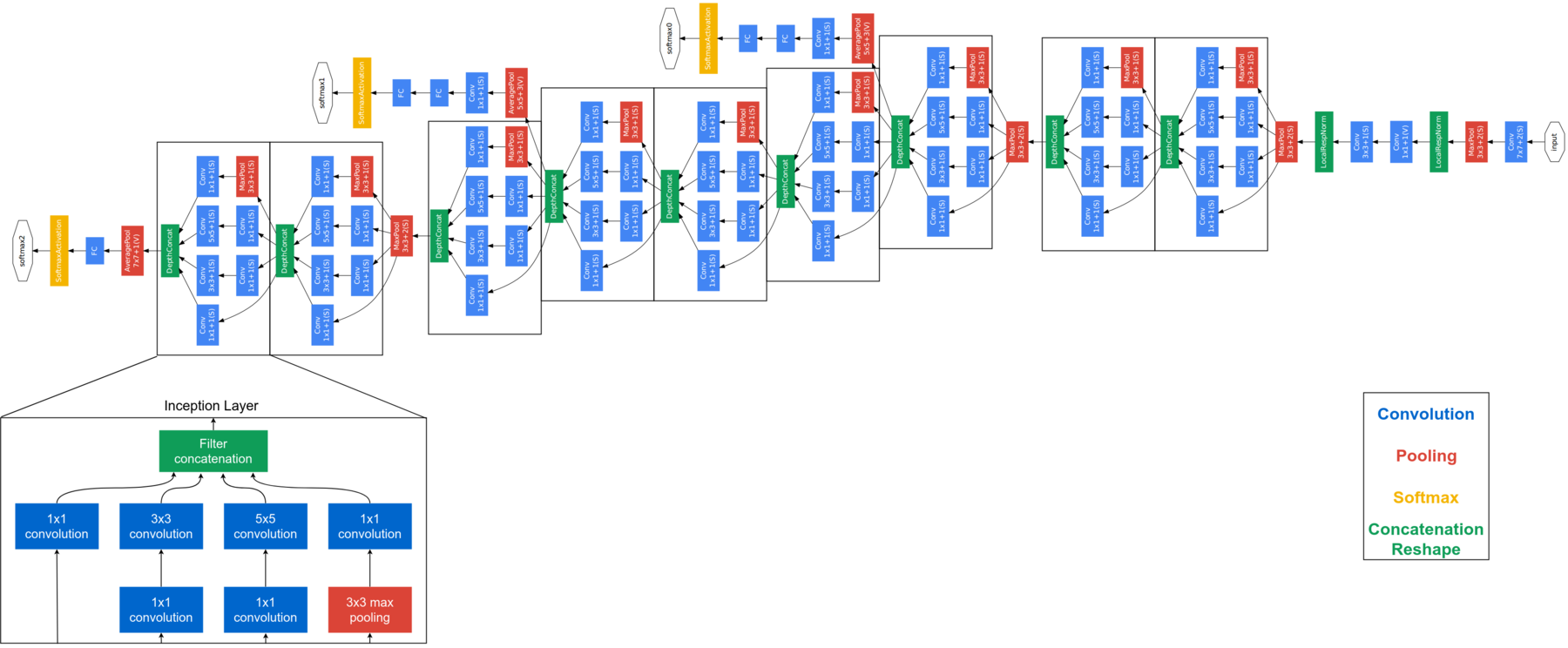
FaceNet is considered to be a state-of-art model developed by Google. It is based on the inception layer, explaining the complete architecture of FaceNet is beyond the scope of this blog. Given below is the architecture of FaceNet. FaceNet uses inception modules in blocks to reduce the number of trainable parameters. This model takes RGB images of 160×160 and generates an embedding of size 128 for an image. For this implementation, we will need a couple of extra functions. But before we feed the face image to FaceNet we need to extract the faces from the images.

detector = dlib.cnn_face_detection_model_v1("../input/pretrained-models-faces/mmod_human_face_detector.dat")

def rect_to_bb(rect):
    # take a bounding predicted by dlib and convert it
    # to the format (x, y, w, h) as we would normally do
    # with OpenCV
    x = rect.rect.left()
    y = rect.rect.top()
    w = rect.rect.right() - x
    h = rect.rect.bottom() - y

    # return a tuple of (x, y, w, h)
    return (x, y, w, h)

def dlib_corrected(data, data_type = 'train'):
    #We set the size of the image
    dim = (160, 160)
    data_images=[]
    #If we are processing training data we need to keep track of the labels
    if data_type=='train':
        data_labels=[]
    #Loop over all images
    for cnt in range(0,len(data)):
        image = data['img'][cnt]
        #The large images are resized
        if image.shape[0] > 1000 and image.shape[1] > 1000:
            image = cv2.resize(image, (1000,1000), interpolation = cv2.INTER_AREA)
        #The image is converted to grey-scales
        gray = cv2.cvtColor(image, cv2.COLOR_BGR2GRAY)
        #Detect the faces
        rects = detector(gray, 1)
        sub_images_data = []
        #Loop over all faces in the image
        for (i, rect) in enumerate(rects):
            #Convert the bounding box to edges
            (x, y, w, h) = rect_to_bb(rect)
            #Here we copy and crop the face out of the image
            clone = image.copy()
            if(x>=0 and y>=0 and w>=0 and h>=0):
                crop_img = clone[y:y+h, x:x+w]
            else:
                crop_img = clone.copy()
            #We resize the face to the correct size
            rgbImg = cv2.resize(crop_img, dim, interpolation = cv2.INTER_AREA)
            #In the test set we keep track of all faces in an image
            if data_type == 'train':
                sub_images_data = rgbImg.copy()
            else:
                sub_images_data.append(rgbImg)
        #If no face is detected in the image we will add a NaN
        if(len(rects)==0):
            if data_type == 'train':
                sub_images_data = np.empty(dim + (3,))
                sub_images_data[:] = np.nan
            if data_type=='test':
                nan_images_data = np.empty(dim + (3,))
                nan_images_data[:] = np.nan
                sub_images_data.append(nan_images_data)
        #Here we add the the image(s) to the list we will return
        data_images.append(sub_images_data)
        #And add the label to the list
        if data_type=='train':
            data_labels.append(data['class'][cnt])
    #Lastly we need to return the correct number of arrays
    if data_type=='train':
        return np.array(data_images), np.array(data_labels)
    else:
        return np.array(data_images)

USING DLIB

DLIB is a widely used model for detecting faces. In our experiments we found that dlib produces better results than HAAR, though we noticed some improvements could still be made:

• If rectangle face bounds move out of the image, we take the whole image instead of the face cropping. It is implemented as follows:
  • if (x>=0 and y>=0 and w>=0 and h>=0):
    • crop_img = clone[y:y+h, x:x+w]
  • else:
    • crop_img = clone.copy()
• For test images, instead of saving one face per image, we are saving all the faces for prediction.
• Rather than a HOG-based detector, we can use a CNN-based detector. As these improvements are tailored to optimize for use with FaceNet, we will define a new corrected face detection.

The above code block extracts the faces from the image, for a lot of images we have multiple faces, so we need to put all those faces in a list. For extracting the faces we are using dlib.cnn_face_detection_model_v1, keep in mind that you should not feed very large dimensional images to this, otherwise you will get a memory error from dlib. If an image doesn’t have a face store NaN in those places. Let’s apply FaceNet to these data images now. The above preprocessing is only needed for test data, train data is already clean which can be seen from the above images. Once we are done obtaining the Face embeddings from train data, get the face embeddings for test data but first, you should use the preprocessing given in the above code block to extract faces from the test data.

def get_embedding(model, face_pixels):
    # scale pixel values
    face_pixels = face_pixels.astype('float32')
    # standardize pixel values across channels (global)
    mean, std = face_pixels.mean(), face_pixels.std()
    face_pixels = (face_pixels - mean) / std
    # transform face into one sample
    samples = expand_dims(face_pixels, axis=0)
    # make prediction to get embedding
    yhat = model.predict(samples)
    return yhat[0]

model = load_model('../input/pretrained-models-faces/facenet_keras.h5')

svmtrainX = []
for index, face_pixels in enumerate(newTrainX):
    embedding = get_embedding(model, face_pixels)
    svmtrainX.append(embedding)

After generating the embeddings for train and test, we are going to use SVM for the classification. Why SVM, you may ask? With a lot of experience, I have come to know that SVM + DL-based features can outperform any other method even Deep learning methods when the amount of data is small.

from sklearn.svm import SVC
from sklearn.pipeline import make_pipeline
from sklearn.naive_bayes import GaussianNB
from sklearn.neural_network import MLPClassifier
from sklearn.preprocessing import StandardScaler, MinMaxScaler, Normalizer

linear_model = make_pipeline(StandardScaler(), SVC(kernel='rbf', C=1.0, gamma=0.01, probability =True))
linear_model.fit(svmtrainX, svmtrainY)

Once the SVM is trained, it’s time to do some testing, but our test data has multiple faces in a list. So, whenever we have Jesse or Mila in an image we will ignore the 0 class and when both Jesse and Mila are present in an image then we’ll choose the one which gives us the higher accuracy.

predicitons=[]
for i in corrected_test_X:    
    flag=0
    if(len(i)==1):
        embedding = get_embedding(model, i[0])
        tmp_output = linear_model.predict([embedding])
        predicitons.append(tmp_output[0])
    else:
        tmp_sub_pred = []
        tmp_sub_prob = []
        for j in i:
            j= j.astype(int)
            embedding = get_embedding(model, j)
            tmp_output = linear_model.predict([embedding])
            tmp_sub_pred.append(tmp_output[0])
            tmp_output_prob = linear_model.predict_log_proba([embedding])
            tmp_sub_prob.append(np.max(tmp_output_prob[0]))
            
        if 1 in tmp_sub_pred and 2 in tmp_sub_pred:
            index_1 = np.where(np.array(tmp_sub_pred)==1)[0][0]
            index_2 = np.where(np.array(tmp_sub_pred)==2)[0][0]
            if(tmp_sub_prob[index_1] > tmp_sub_prob[index_2] ):
                predicitons.append(1)
            else:
                predicitons.append(2)
        elif 1 not in tmp_sub_pred and 2 not in tmp_sub_pred:
            predicitons.append(0)
        elif 1 in tmp_sub_pred and 2 not in tmp_sub_pred:
            predicitons.append(1)
        elif 1 not in tmp_sub_pred and 2 in tmp_sub_pred:
            predicitons.append(2)

DISCUSSION

Final remarks, this is a very small dataset so results can change hugely even with adding or deleting even a few images. In our test we found that it fooled us many times, there were around 20 images in the test which were predicted wrongly by us but correctly by our model. We confirmed the predicted result by searching those images on google.

Deep neural networks are able to extract more meaningful features than machine learning models. The downfall of these big networks is however the need for a huge amount of data. We managed to cope with this issue by using a pre-trained model, a model that has been trained on a way bigger dataset in order to retain knowledge on how to encode face images, which we then used for our purposes in this challenge. In addition, fine-tuning SVM really helped us to push beyond the accuracy of 95%.